Usage manual
Load genomic annotations and input files
Running offline
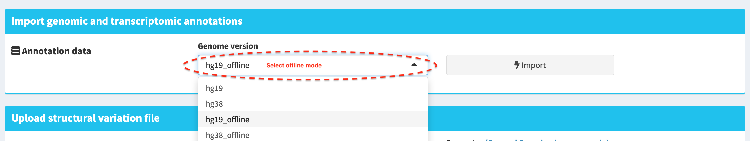
By default, the initiation of IGV browser in FuSViz linear module needs an online environment. However, with some additional configurations, it is able to run FuSViz on an offline system. Users will need to manually upload pre-defined genome reference and index files, and cytoband annotation for launching the IGV session.
For human genome version hg19:
For human genome version hg38 (files need to be renamed or unzipped after downloading):
hg38.fasta (renamed after download) - https://s3.amazonaws.com/igv.broadinstitute.org/genomes/seq/hg38/hg38.fa
hg38.fasta.fai (renamed after download) - https://s3.amazonaws.com/igv.broadinstitute.org/genomes/seq/hg38/hg38.fa.fai
cytoBandIdeo.txt (unzip after download) - https://s3.amazonaws.com/igv.org.genomes/hg38/annotations/cytoBandIdeo.txt.gz
Select an offline mode in
Genome versionbox
Upload a genome reference (e.g. hg19.fasta), an index file (e.g. hg19.fasta.fai) and a cytoband annotation (e.g. cytoBand.txt) via
Upload a filebox in linear module
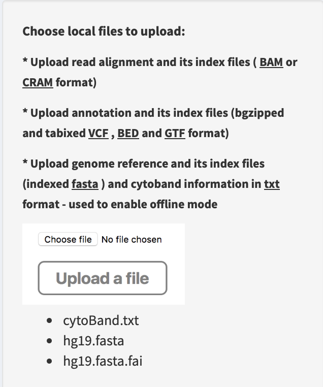
Load gene annotation track, i.e. press
Load gene track (offline)button in Linear module
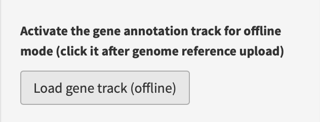
Now, the offline IGV browser session is launched successfully (for the usage, see Linear module section below).
FuSViz annotation resources
Annotations of human genome version (hg19 and hg38) and mouse genome version (GRCm39) are provided, and they include:
The gene, transcript and exon annotations (ENSEMBL Release 104 gene annotation on reference chromosomes for hg38, ENSEMBL Release 87 gene annotation on reference chromosomes for hg19, ENSEMBL Release 111 gene annotation on reference chromosomes for GRCm39). NOTE: scaffolds and contigs are excluded in FuSViz analysis.
Gene symbol and synonymous names - the resource for approved human gene nomenclature HGNC were downloaded using ENSEMBL BioMart API service
Protein domains and motifs are from InterPro database v86. NOTE: InterPro integrates signatures of several databases (e.g. CDD, Pfam, SMART, Prosite and MobiDB). In terms of different sources, domain length, structure and name may be incongruous. Domains with overlapping intervals are merged and the most common name represents its entry.
Literature-mined database of tumor suppressor genes/proto-oncogenes – CancerMine v42. NOTE: status of proto-oncogenes and tumor suppressor genes are determined according to the following rule:
A given gene with a support of at least two literatures that suggest an oncogenic or tumor suppressor role.
A one-way fisher exact test is performed on the number of literatures with an evidence as proto-oncogene or tumor suppressor gene. If
pvalue <= 0.05,0.05 < pvalue < 0.95andpvalue >= 0.95, oncogene, cancer-related gene or tumor suppressor gene is tagged, respectively.Proto-oncogenes/tumor suppressor candidates from CancerMine that were found in the curated list of false positive cancer drivers defined by Bailey et al, Cell 2018 are excluded.
Drug target entry association with cancer from Open Targets Platform - Database of molecularly targeted drugs and tractability aggregated from multiple sources (literature, pathways and mutations), release 2022-02-01.
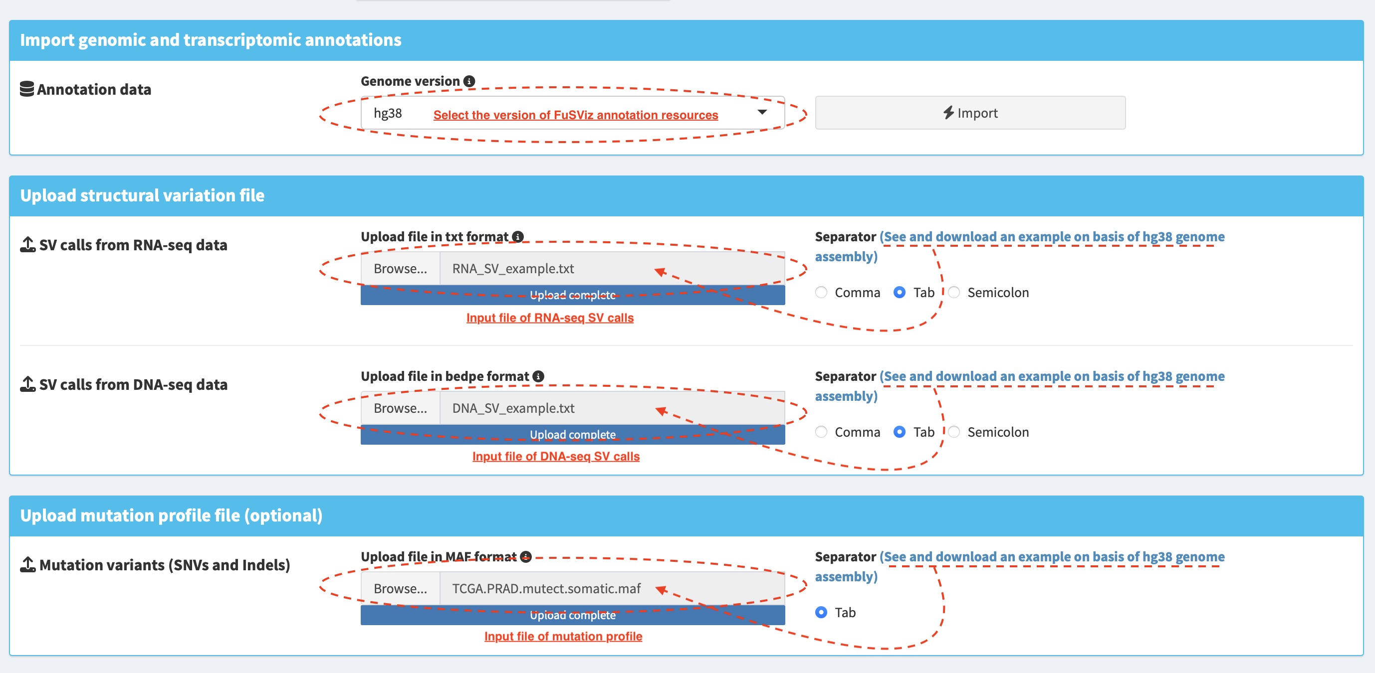
Import SV and mutation files
See Input section - requisite input format for FuSViz and how to
prepare the input file.
Table overview of import data
Import RNA and DNA SV calls and mutation profile are demonstrated in tab
panels SV from RNA-seq, SV from DNA-seq and
Mutation profile, respectively.
Table – sorting, filtering and prioritizing SVs
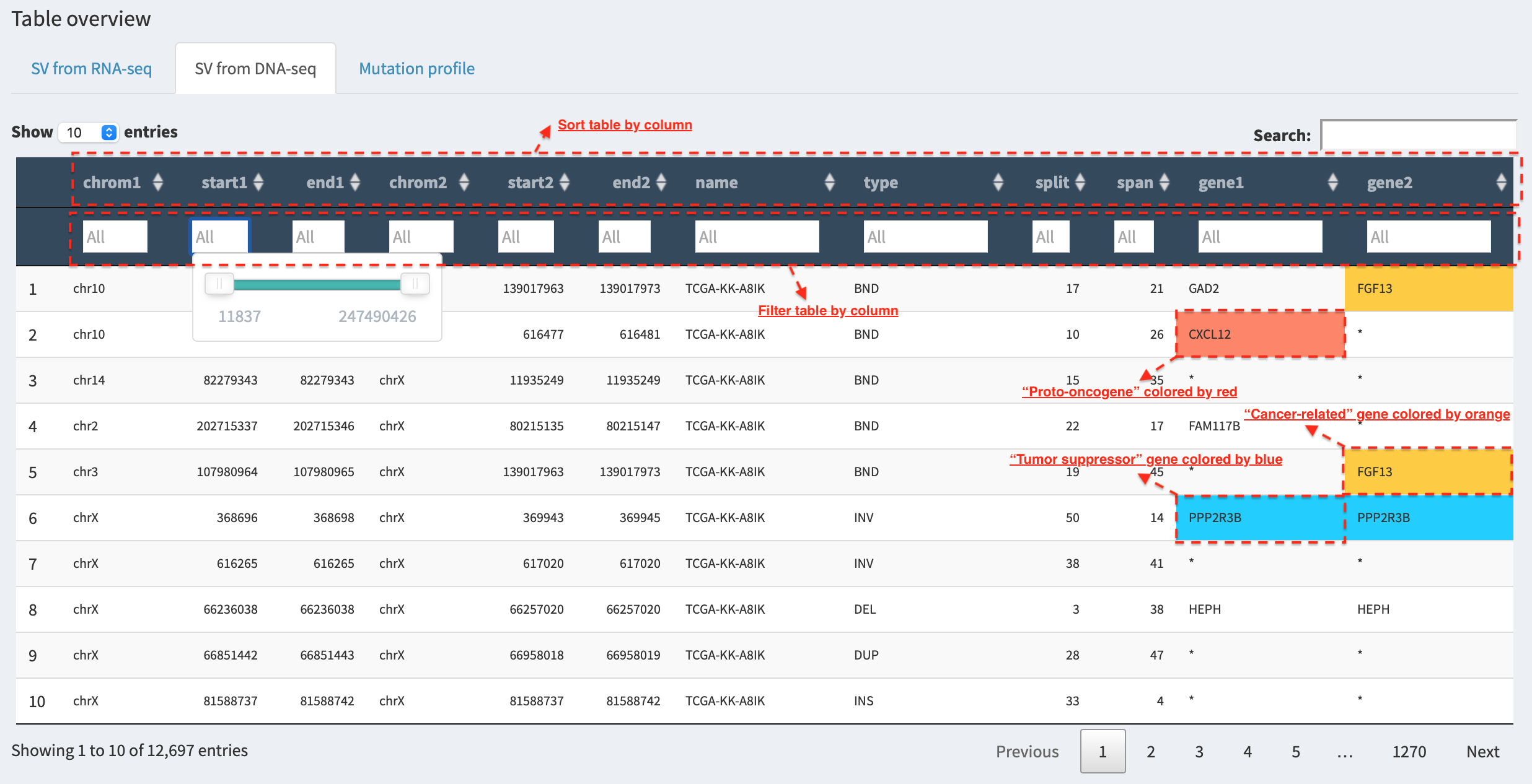
For example, in SV from DNA-seq tab panel, genes involved in SVs are
highlighted by red, blue and orange if they are
proto-oncogenes, tumor suppressor genes and cancer-related genes.
Table – save the updated table
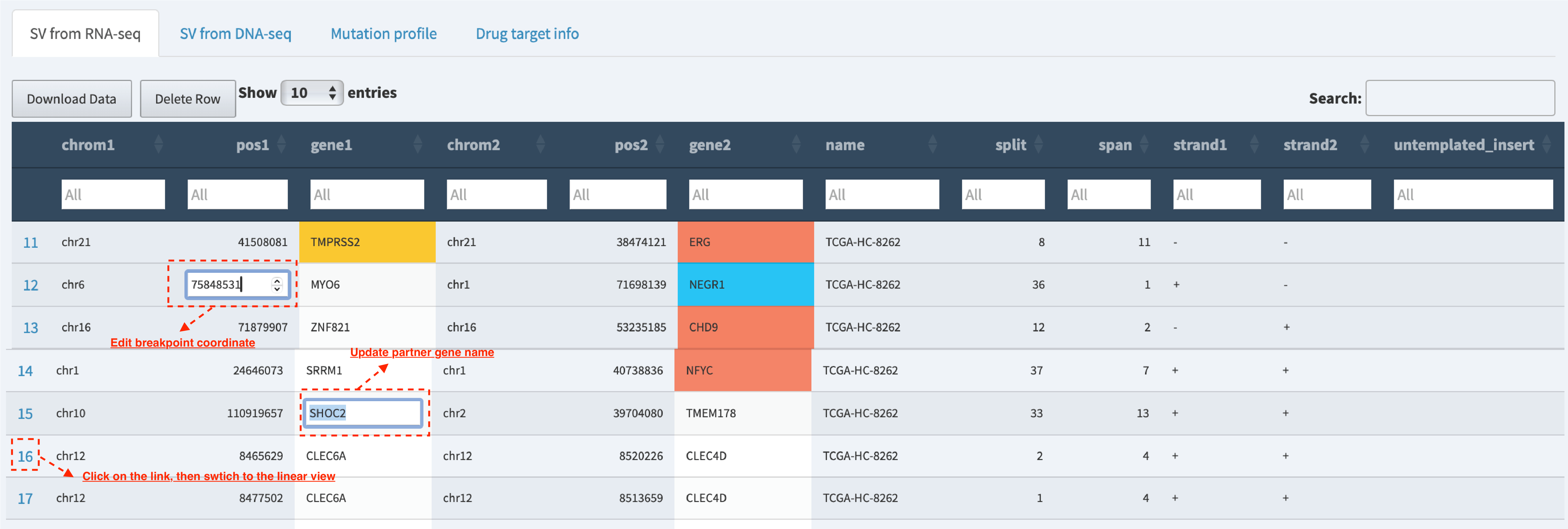
Users are allowed to edit and update the SV data in table view session (e.g., correct the breakpoint coordinates if the provisional one proves inaccurate, update gene symbol name if necessary and add a comment on the quality of SV).
Table – edit and update data
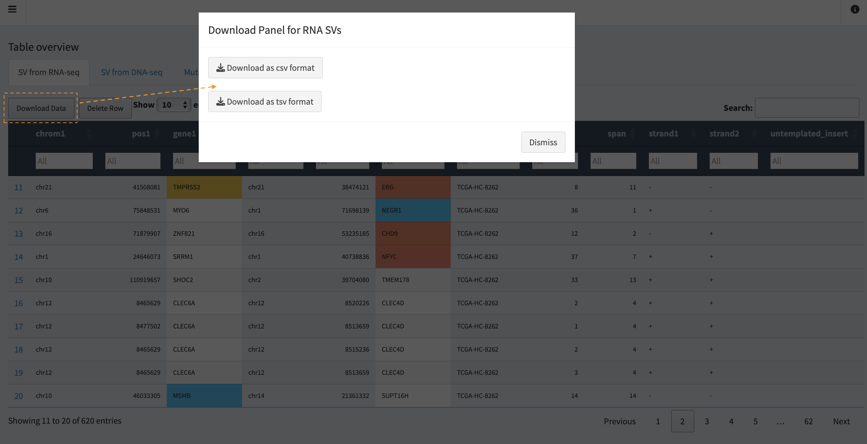
Users are able to output the updated and reviewed SV table into a text
file, by clicking on the Download Data button.
Wordcloud – prevalence of SV-related genes across samples
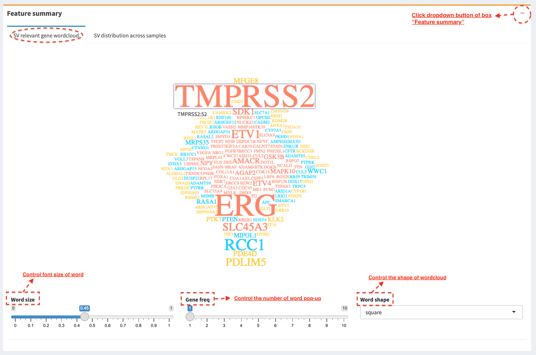
In SV relevant gene wordcloud tab panel, a pop-up window shows the
frequency of SV partner genes in sample cohort (e.g. TMPRSS2: 52)
after mouse over a word. Font size of a word is adjusted via
Word size slider; the number of words displayed in the layout is
controlled via Gene freq slider (words with a frequency < selected
value are filtered out); shape of wordclould is customized via
Word shape select box (options: ‘circle’, ‘square’ and ‘cardioid’).
Histogram – SV distribution across samples
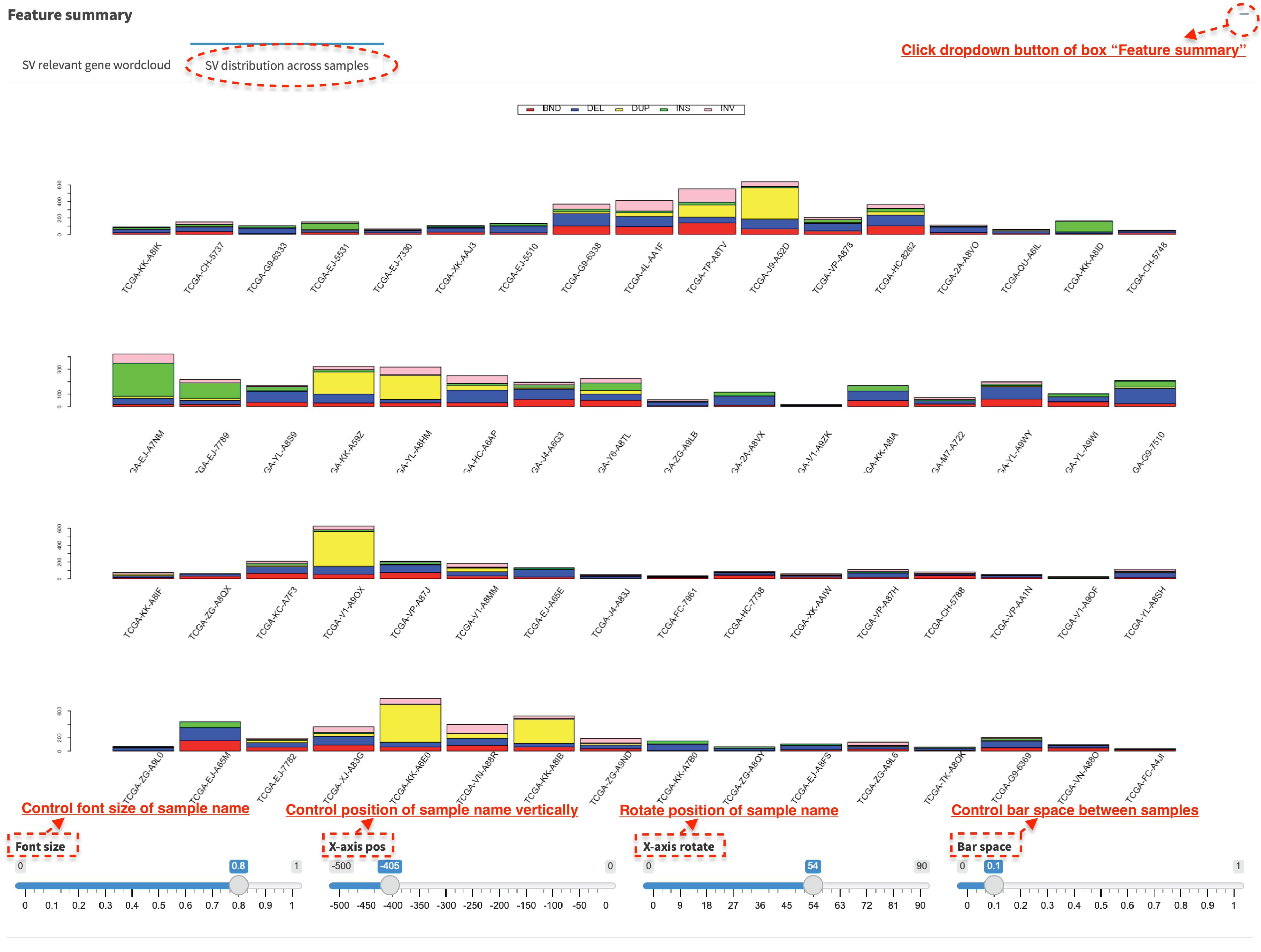
In SV distribution across samples tab panel, histogram plots the
number of SVs per sample, which is used to identify any hyper-SV
samples. For SV calls from DNA-seq data, the frequency of each SV type
per sample is plotted and it shows a distribution of SVs to different
categories. Font size of sample name is adjusted via Font size
slider; position of sample name can be changed vertically via
X-axis pos slider; position of sample name is rotated via
X-axis rotate slider; bar space between samples is controlled via
Bar space slider.
Correlation - small variant mutations and SVs burden
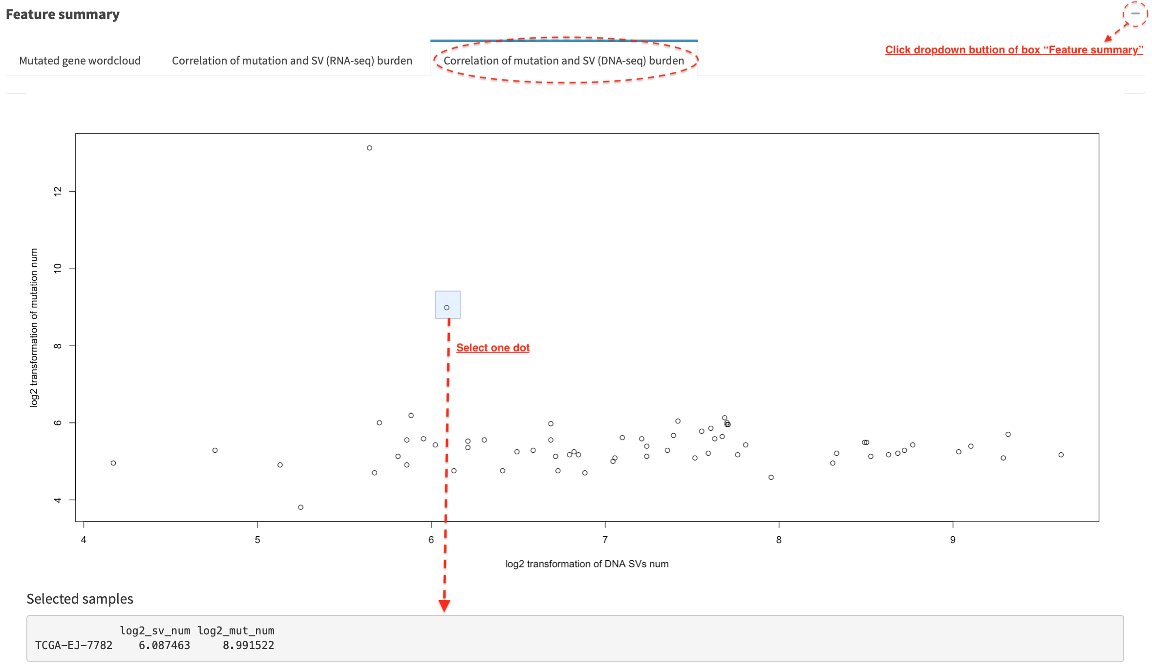
In Correlation of mutation and SV (DNA-seq) burden tab panel, the
relationship between small variant and SV burden is plotted if mutation
profile is available. Mutation and SV burden of a selected sample
(e.g. dot in a dashline box) is shown in a table below (the value is
log2 transformed).
Drug target association with cancer-related genes
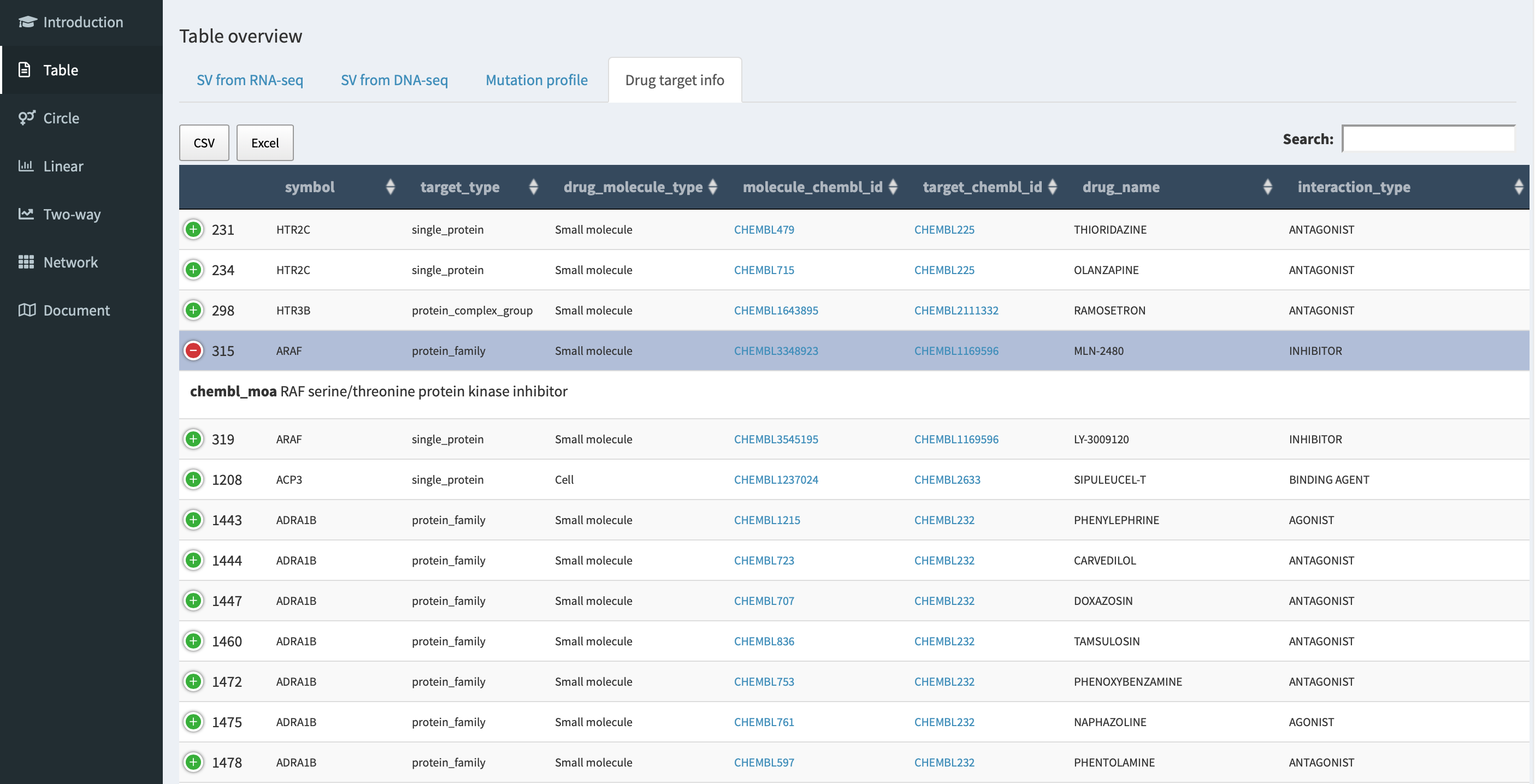
In Drug target info tab panel, genes involved in RNA-seq/DNA-seq SVs
with an entry in Open Targets
Platform database are listed in a
table with drug targeting annotation (e.g. molecular_chembl_id -
available antineoplastic drug with
ChEMBL compound identifier;
target_chembl_id - ChEMBL
compound identifier of the targeted gene; interactive_type - an
interactive way of drug to the target gene).
Circular module
Circular plot analyses of RNA-seq and DNA-seq SVs are demonstrated in
RNA_SV_circular_plot and DNA_SV_circular_plot tab panels,
respectively.
Whole genome SVs overview
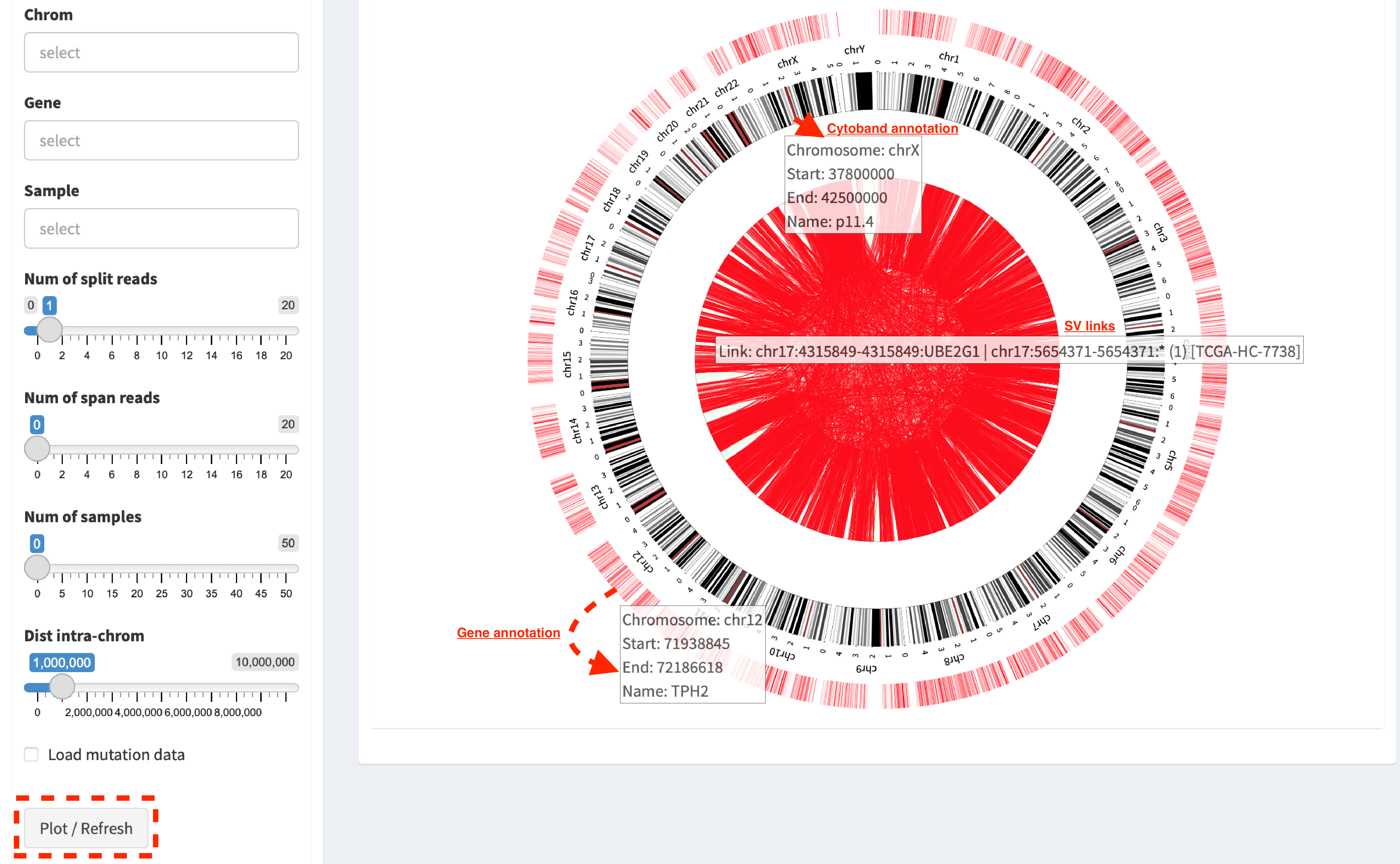
Press button Plot / Refresh. Circular tracks displayed from
outermost to innermost are Gene annotation, Cytoband annotation
and SV links. For a pop-up window of one SV link (after mouse over),
it shows as
Link: chr17:4315849-4315849:UBE2G1 | chr17:565471-565471:* (1) [TCGA-HC-7738],
i.e. the breakpoint of UBE2G1 at chr17:4315849 is linked to the
breakpoint of an intergenic region (marked by *) at chr17:565471, and
it is present in one sample (TCGA-HC-7738).
Demo SVs with customized settings
Users could make a change on the settings of RNA_SV_panel or
DNA_SV_panel for a customized analysis.
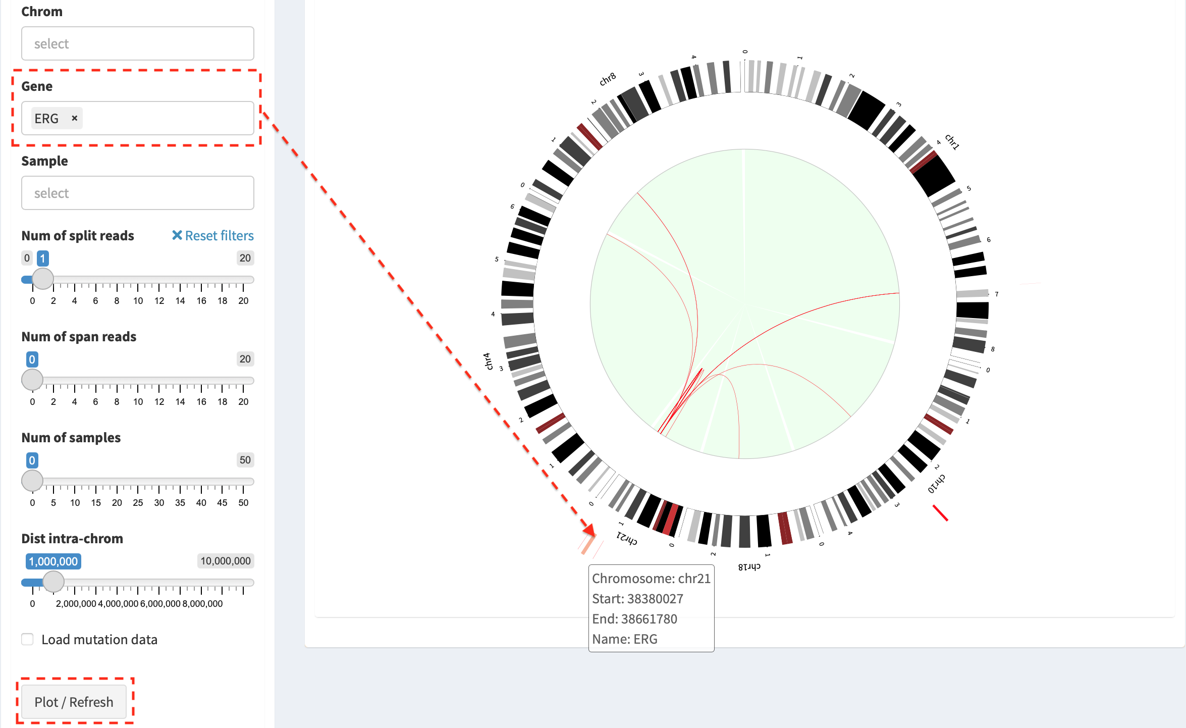
Press button Plot / Refresh after selecting Gene ERG. SV
events of ERG gene and the relevant chromosomes (e.g. chromosome 1, 4,
8, 10, 18 and 21) are plotted. More customized investigations could be
done by choosing in Chrom or Sample box.
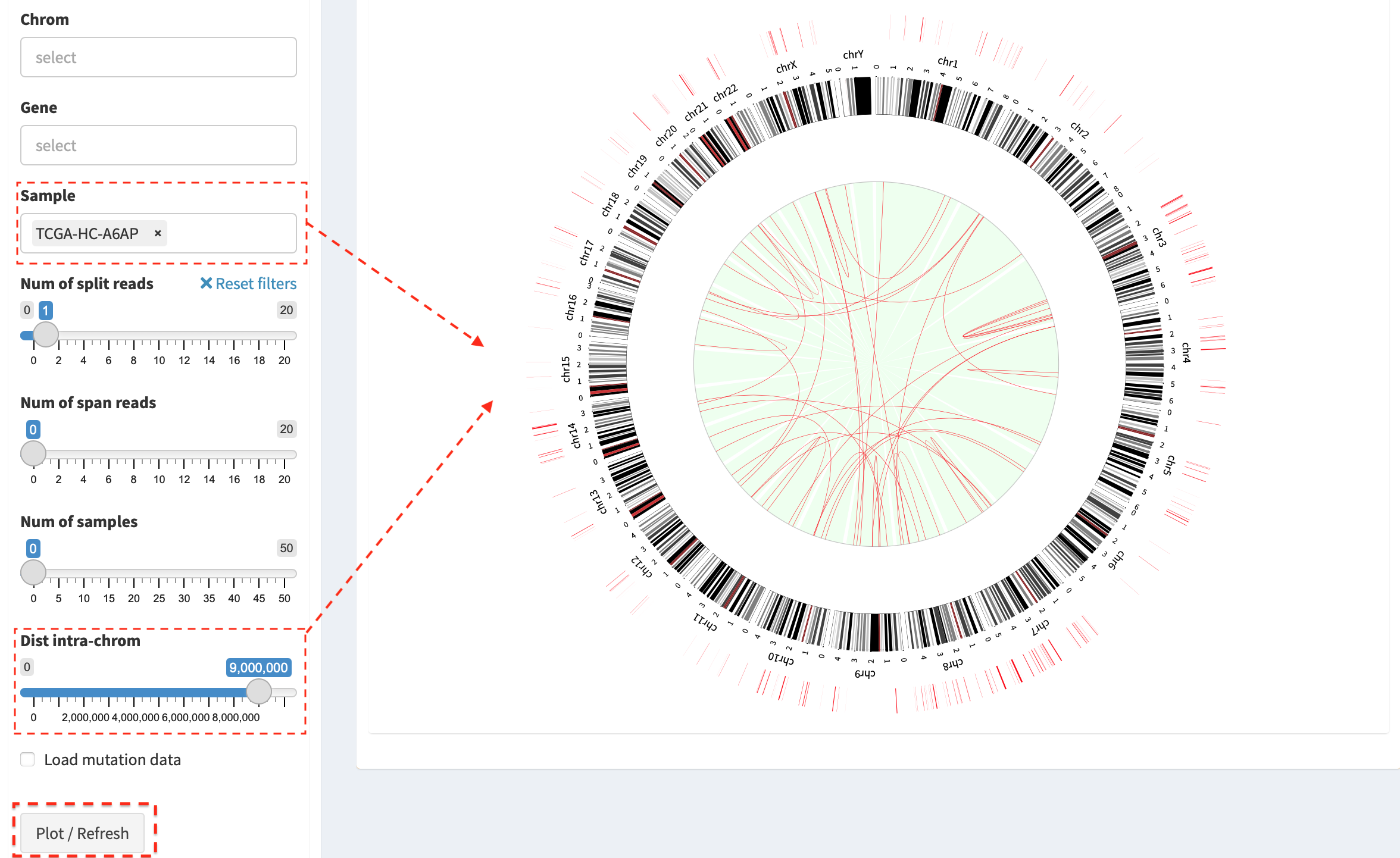
Another example - an overview of filtered SVs (intra-chromosome SVs with
a distance > 9Mb are kept) in sample “TCGA-HC-A6AP”. NOTE: slider
Dist intra-chrom is used for filtering out intra-chromosome SV
events with a distance less than a given value.
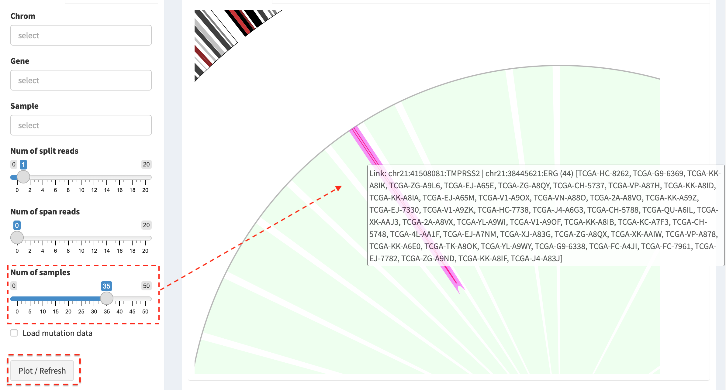
By changing the value of Num of samples slider, the most recurrent
SVs (>35 samples) in the cohort of samples are displayed.
Integrate SVs and mutation data
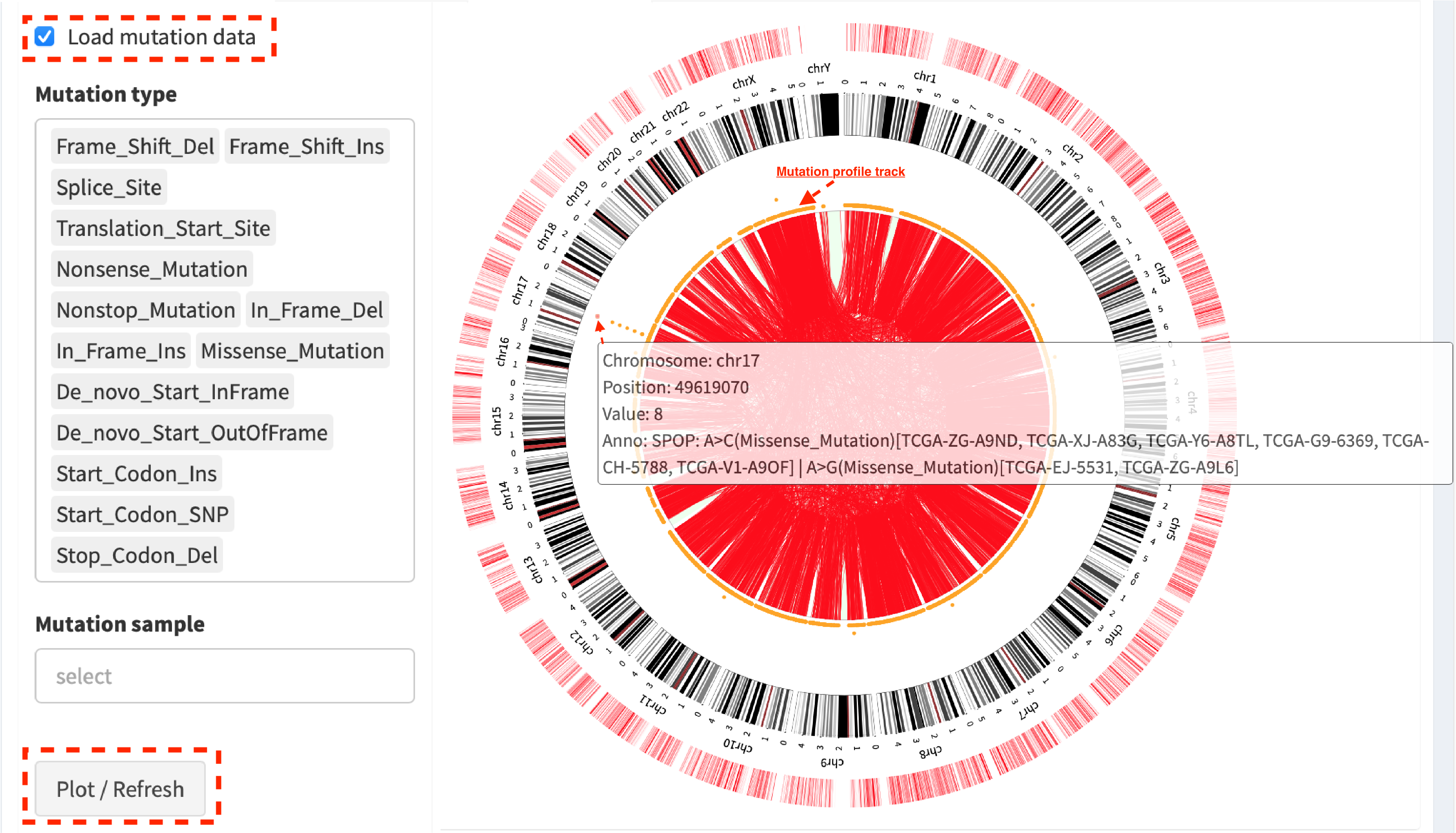
Click check box Load mutation data (by default, mutation types with
no-silent consequence are chosen in Mutation type; leave it to be
empty if all mutation types are included), then click button
Plot / Refresh. Mutation profile track is added between
Cytoband annotation and SV links tracks. An example shows:
Chromosome:17 Position:49619070 Value:8 Anno:SPOP: A>C(Missense_Mutation)[TCGA-ZG-A9ND, TCGA-XJ-A83G, TCGA-Y6-A8TL, TCGA-G9-6369, TCGA-CH-5788, TCGA-V1-A9OF] | A>G(Missense_Mutation)[TCGA-EJ-5531, TCGA-ZG-A9L6]
It denotes that eight samples have a mutation variant at the genomic position “chromosome 17:49619070”, in which two different missense mutations (A>C and A>G) are distributed in six and two samples, respectively.
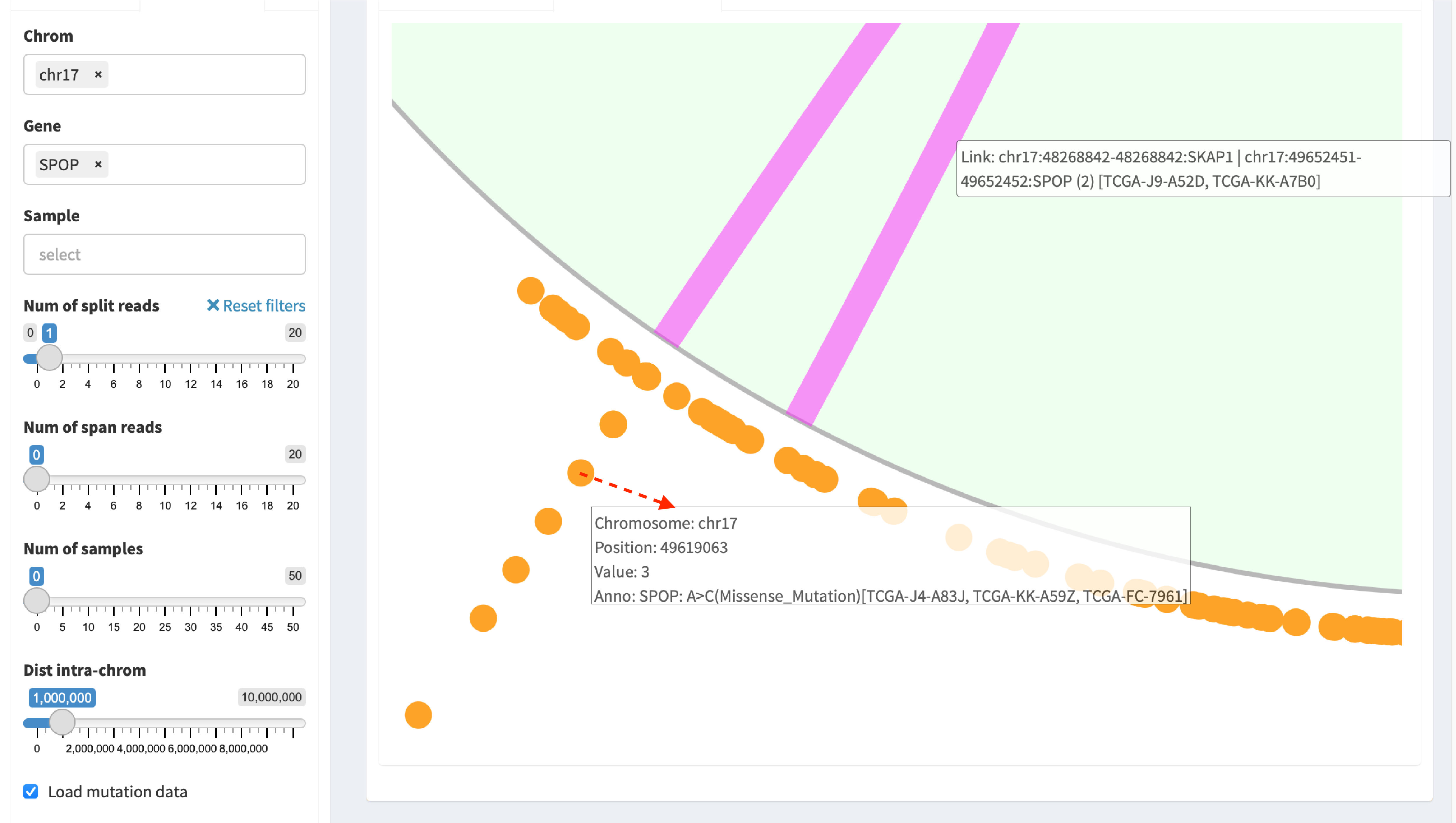
Zoom-in circular plot
Two options are available for zooming in: spinner of the mouse or
double-click a targeted object. For example, double-click a mutation
dot (marked by arrow line) in the plot for zooming in:
Download circular plot
Press Download circular plot, and current page is saved as a
htmlwidget.
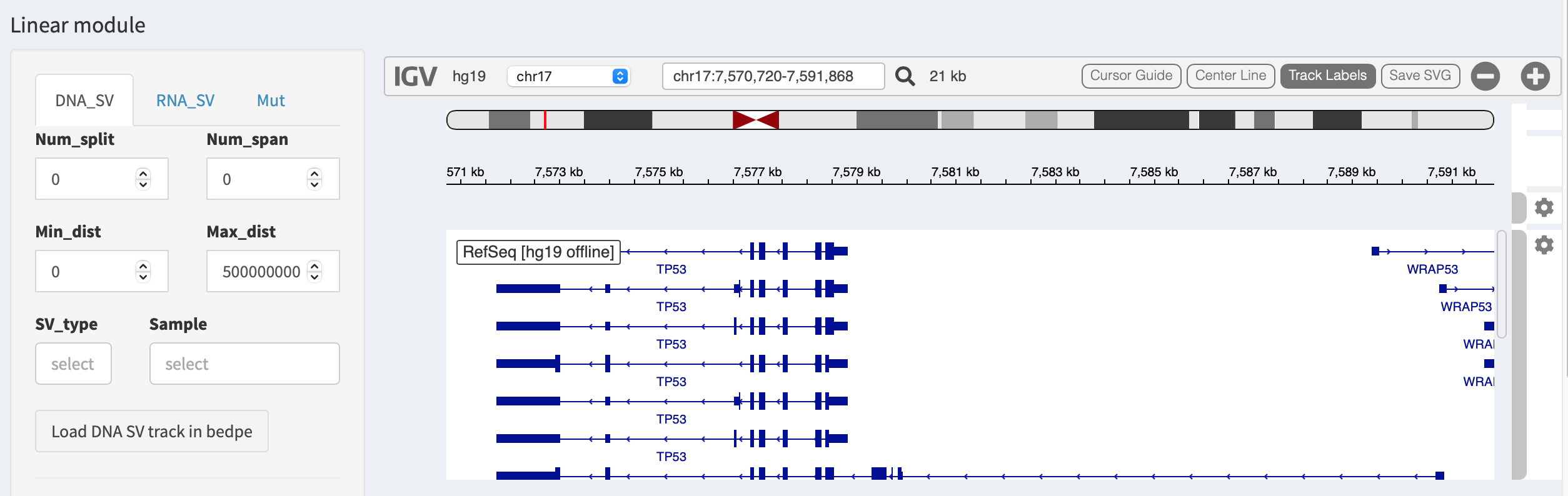
Linear module
Linear module is built on basis of an embeddable interactive genome
visualization Javascript library
igv.js. A htmlwidget is created
to communicate between R and Javascript, and render the functionality of
igv.js. By default, IGV browser
interface is automatically launched by selecting a genome reference
version (hg19 or hg38) in
Import genomic and transcriptomic annotations of Introduction page.
SVs can be loaded in different types of genomic tracks and are
illustrated per each chromosome. FuSViz accepts four types of tracks
(i.e. bedpe, segment, bed and bedgraph formats). Users
could configure the setting of loaded tracks in SV_DNA, SV_RNA
and Mut panels.
Load SVs in “bedpe” format (available for DNA-seq and RNA-seq SVs)
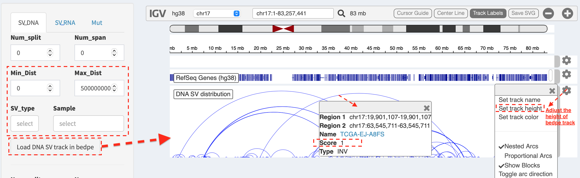
Press Load and refresh DNA SV track in bedpe button,
intra-chromosome SVs are denoted as curves that link breakpoint sites.
After clicking a curve, a window pops up with a feature description of
the selected SV, e.g.
Region1: chr17 19901107-19901107- breakpoint site/interval of first end of SVRegion2: chr17 63545711-63545711- breakpoint site/interval of second end of SVName: TCGA-EJ-A8FS- sample nameScore: 1- the number of samples has this SVType: INV- SV type as inversion
Some options in the panel are used to filter and prioritize SVs
(e.g. Min_Dist and Max_Dist for filtering out SV with a distance
out of a given range; SV_type and Sample for prioritizing SVs of
selected types or samples). Users can adjust the layout of bedpe track
via configuration panel (e.g. Set track height).
Load SVs in “segment” format (only available for DNA-seq SVs)
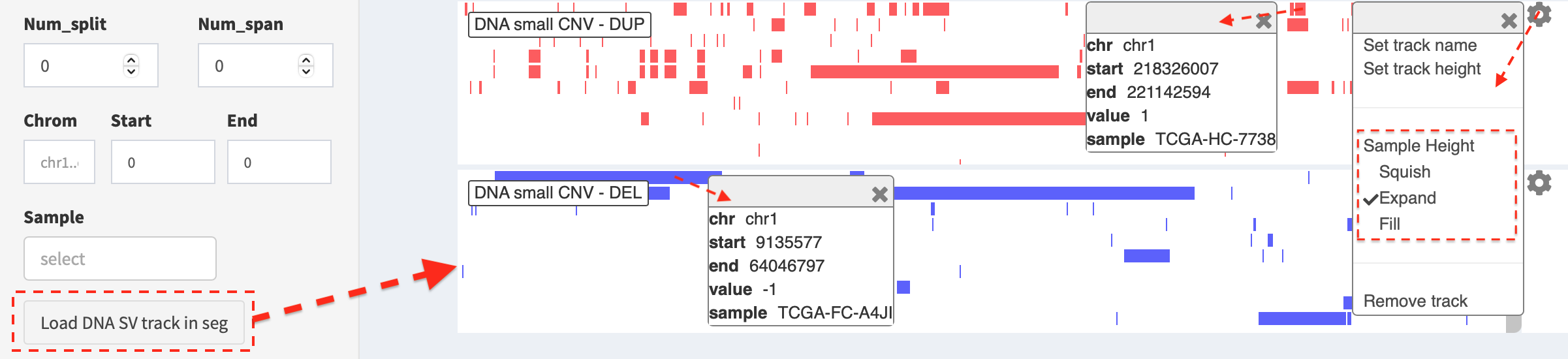
Press Load and refresh DNA SV track in seg button, two types of SVs
(i.e. duplication and deletion) representing copy number
aberrations (CNAs) are displayed, in which duplication and
deletion of genomic segments are colored by red and blue
bars, respectively. A window pops up with a feature description of the
clicked bar, e.g.
chr: chromosome- chromosome namestart: 218326007- start coordinate of segment intervalend: 221142594- end coordinate of segment intervalvalue: 1(duplication) /-1(deletion)sample: TCGA-HC-7738- sample name
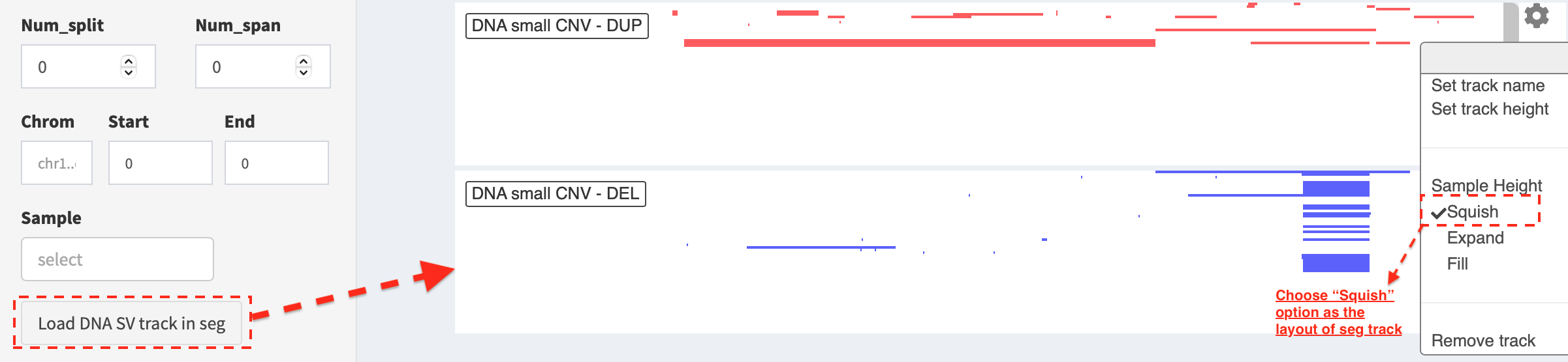
Here, the layout of seg track is set as Expand mode (default value)
in the configuration and user is able to choose Squish option to
show duplication and deletion events in a compact way. For a
customized adjustment of the track size, it can be done via
Set track height setting. An example below,
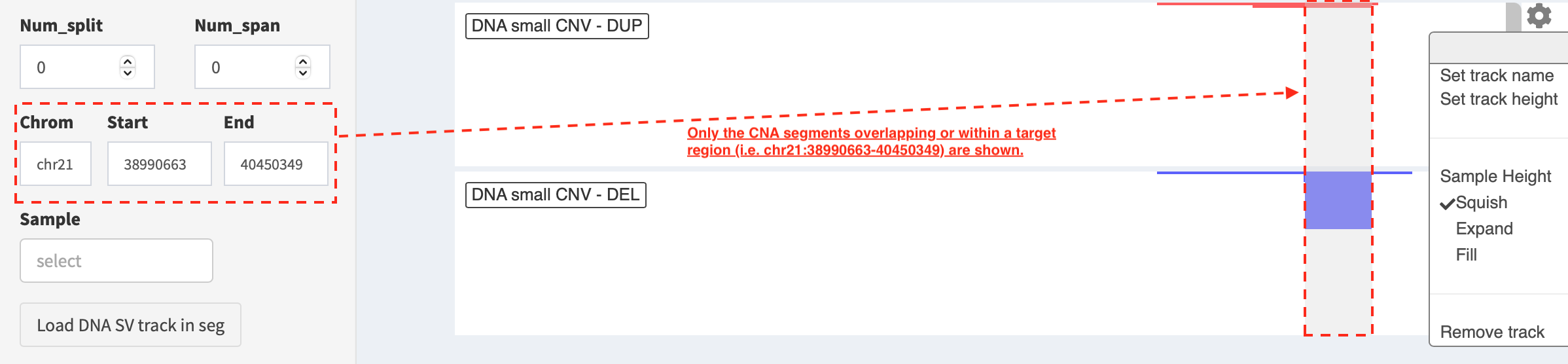
If users are interested in CNAs overlapping/within a target region, a
subset of duplication and deletion are displayed by the setting
of Chrom, Start and End options
(e.g. “chr21:38990663-40450349”) in SV_DNA panel.
Load SVs in “bed” and “bedgraph” format (available for DNA-seq and RNA-seq SVs)
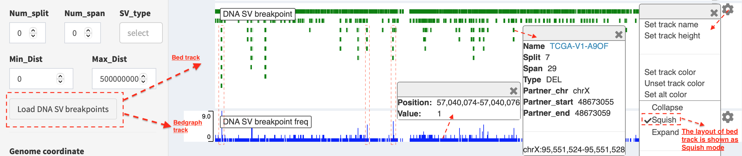
Press Load and refresh DNA breakpoints in bed (or
Load and refresh RNA breakpoints in bed) button, SV breakpoint
tracks in bed (upper – colored by green) and bedgraph (below –
colored by blue) format are loaded together. In bed format track, a
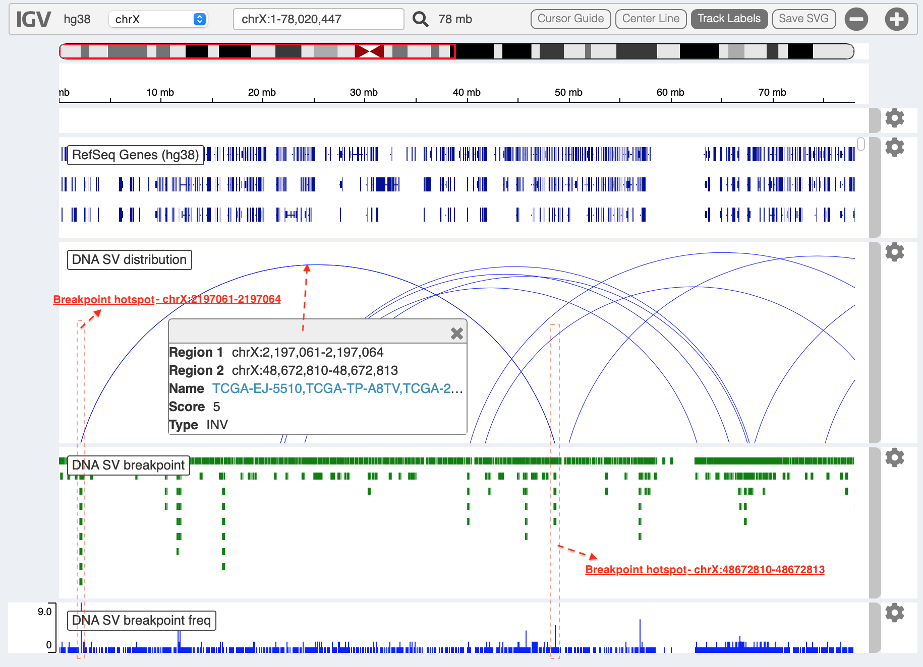
window pops up after clicking a breakpoint:
Name: TCGA-V1-A9OF- sample namesplit: 7- the number of split read supportspan: 29- the number of discordant read pair supportType: DEL- SV type as deletionPartner_chr: chrX- the chromosome on which the other breakpoint of SV is locatedPartner_startandPartner_end: 48673055 and 48673059- the zero-based starting and one-based end position of the other breakpoint of the SV onPartner_chrchrX: 95551524-95551528- the chromosome, zero-based starting and one-based end position of the clicked SV breakpoint
Bedgraph tracks display the frequency of recurrent breakpoints across
samples. After clicking one peak, the frequency (e.g. value: 1) of a
breakpoint (e.g. Position: 57040074-57040076) is shown in a pop-up
window.
Bed and bedgraph tracks could be used for an identiification of
breakpoint hotspot regions (see breakpoint hotspots highlighted in
dashline boxes, which links a recurrent inversion between
chrX:2197061-2197064 and chrX:48672810-48672813).
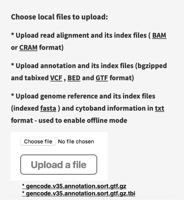
Upload user-defined annotation files
Users are allowed to upload customized annotation files in VCF (e.g. genetic variations), BED (e.g. regulatory elements - enhancers and TADs) and GTF (e.g. genes, transcripts, exons) formats to interpret SV patterns. Some requirements of a customized annotation file:
Chromosome name MUST start with “chr”
All upload files MUST be sorted by chromosome and genomic coordinate, then compressed and indexed using bgzip and tabix
The compressed file MUST upload together with its index file
Make sure genomic coordinate in upload annotation files MUST be the same version as used in IGV browser
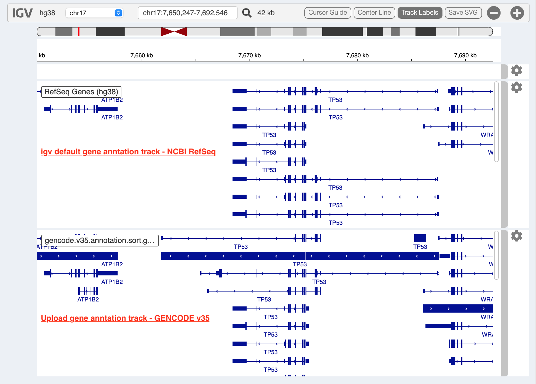
For example, upload a gene annotation file in GTF format from GENCODE v35 and compare it with the default annotation track (NCBI RefSeq).
In addition, read alignment files (e.g. BAM or CRAM format) can be uploaded for a single sample analysis (see Appendix section for usage and case example).
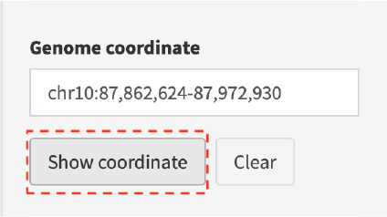
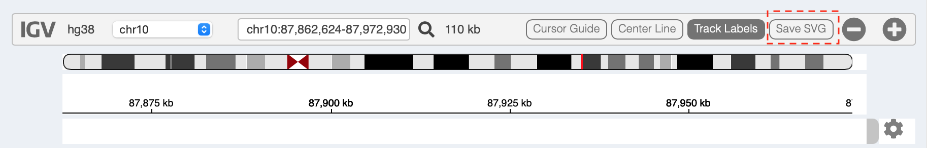
Display genomic coordinate of current window
Press Show coordinate button
Save and download tracks
IGV browser provides a button Save SVG to download loaded tracks as
SVG format.
Illustrate SV pattern by combining multiple tracks together
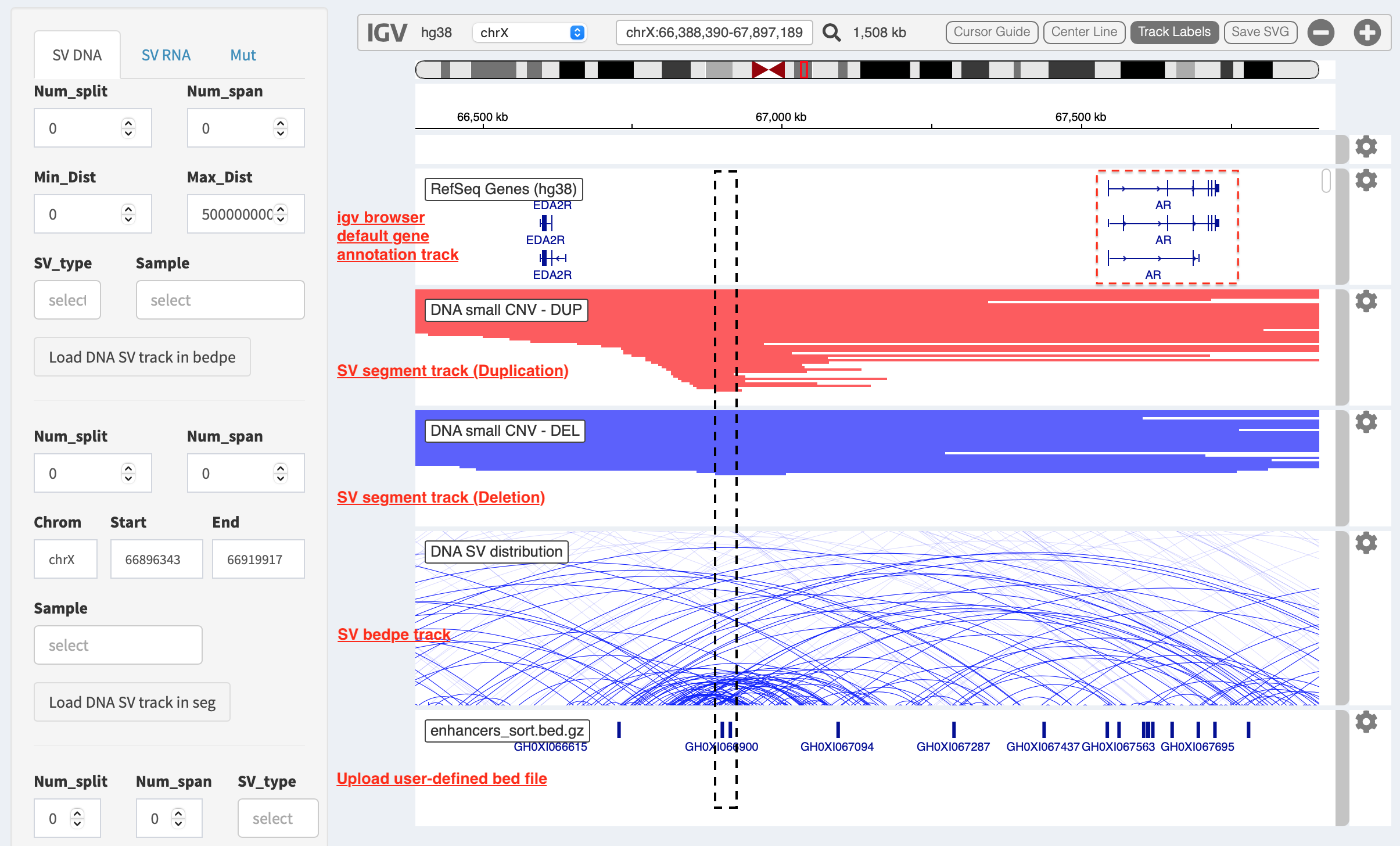
Example 1: identify recurrent duplications involving an upstream enhancer of AR gene
Loaded tracks from the top denote chromosome ideogram, gene annotation (NCBI RefSeq), SV in segment format (duplication and deletion), SV in bedpe format and user-defined bed file (enhancers_sort.bed.gz). Dashline box highlights a highly recurrent duplication of an upstream enhancer GHXI66900 for AR gene in a sample cohort.
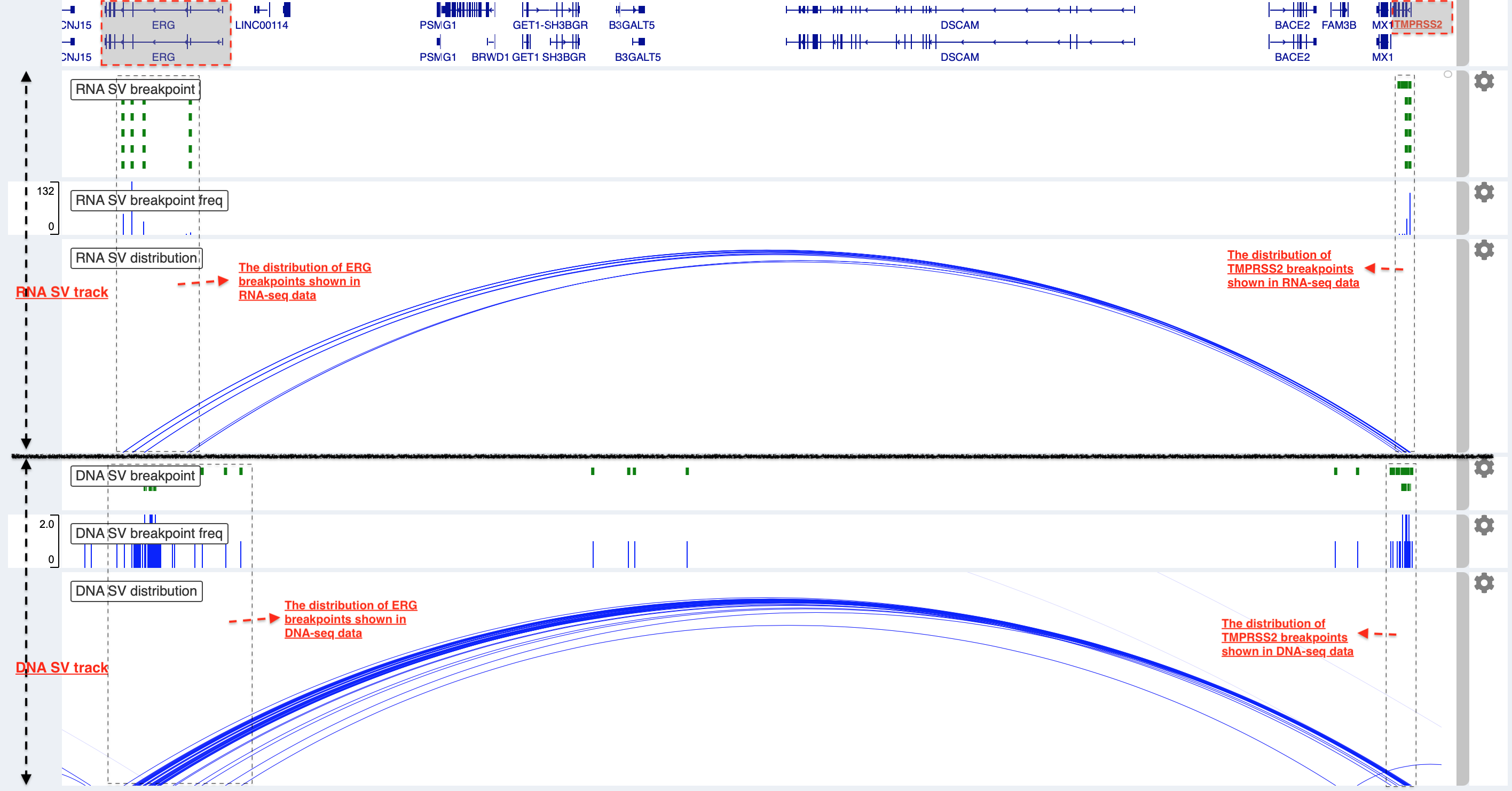
Example 2: a comparison of breakpoint distribution at DNA and RNA level
In loaded SV tracks from DNA-seq data, breakpoints within TMPRSS2 and ERG (highlighted in grey boxes) show a scatter distribution, and no peak indicates a high recurrence. While the observed breakpoints of these two genes at RNA level are centralized at a few exon-exon boundaries with a high recurrence. As introns mostly conbritue to a gene composition in length and are therefore enriched in breakpoints compared to exons, RNA splicing mechanism make most transcribed breakpoints aligned to exon boundary, simplifying the complexity of SVs in the RNA-seq data. As expected in bedpe track, fusion events of TMPRSS2-ERG detected in RNA-seq data link the splicing sites of two partner genes.
Two-way module (RNA-seq)
Two-way module is designed for an analysis of a specific SV type
(i.e. fusion gene/transcript) in a single panel, where two distant
genomic intervals involved in a few fusion events are shown together
with gene annotations. Three functional panels (i.e. Overview_plot,
Sample_plot and Domain_plot) are provided to investigate fusion
events in different dimensions.
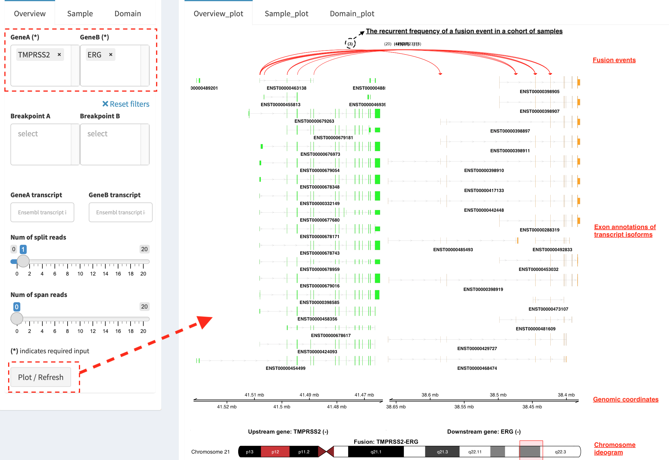
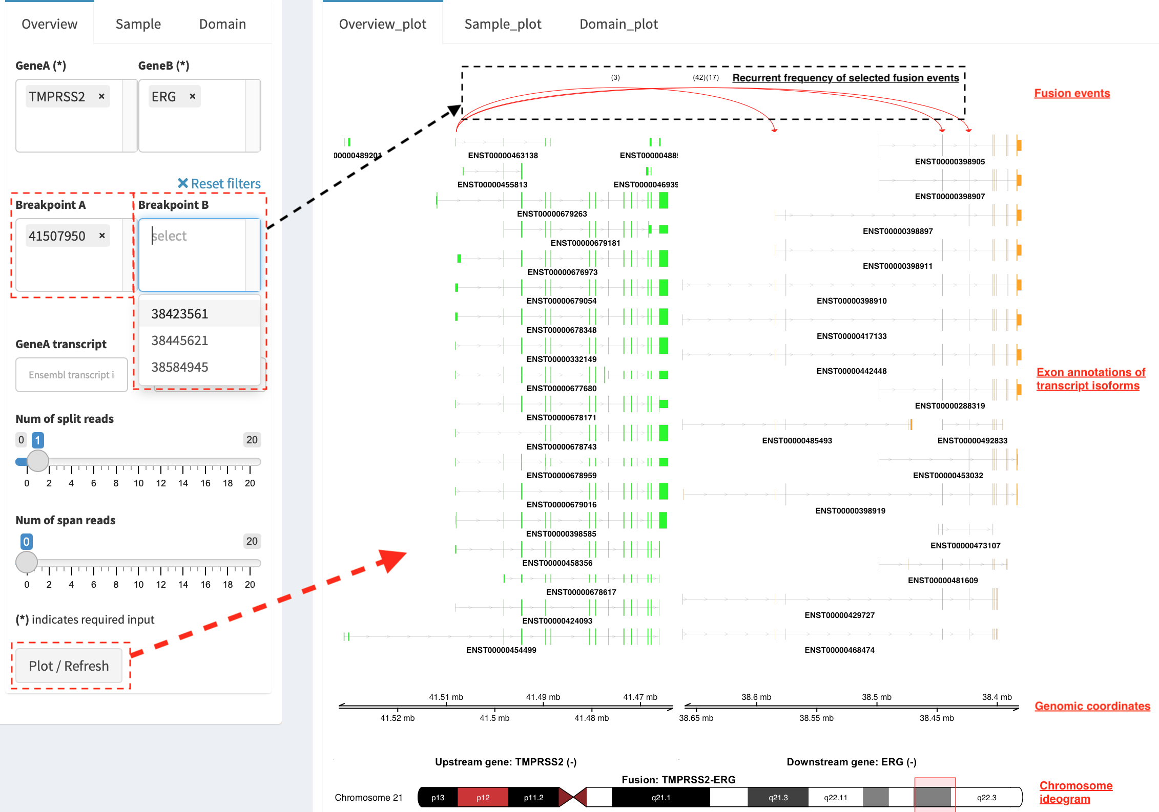
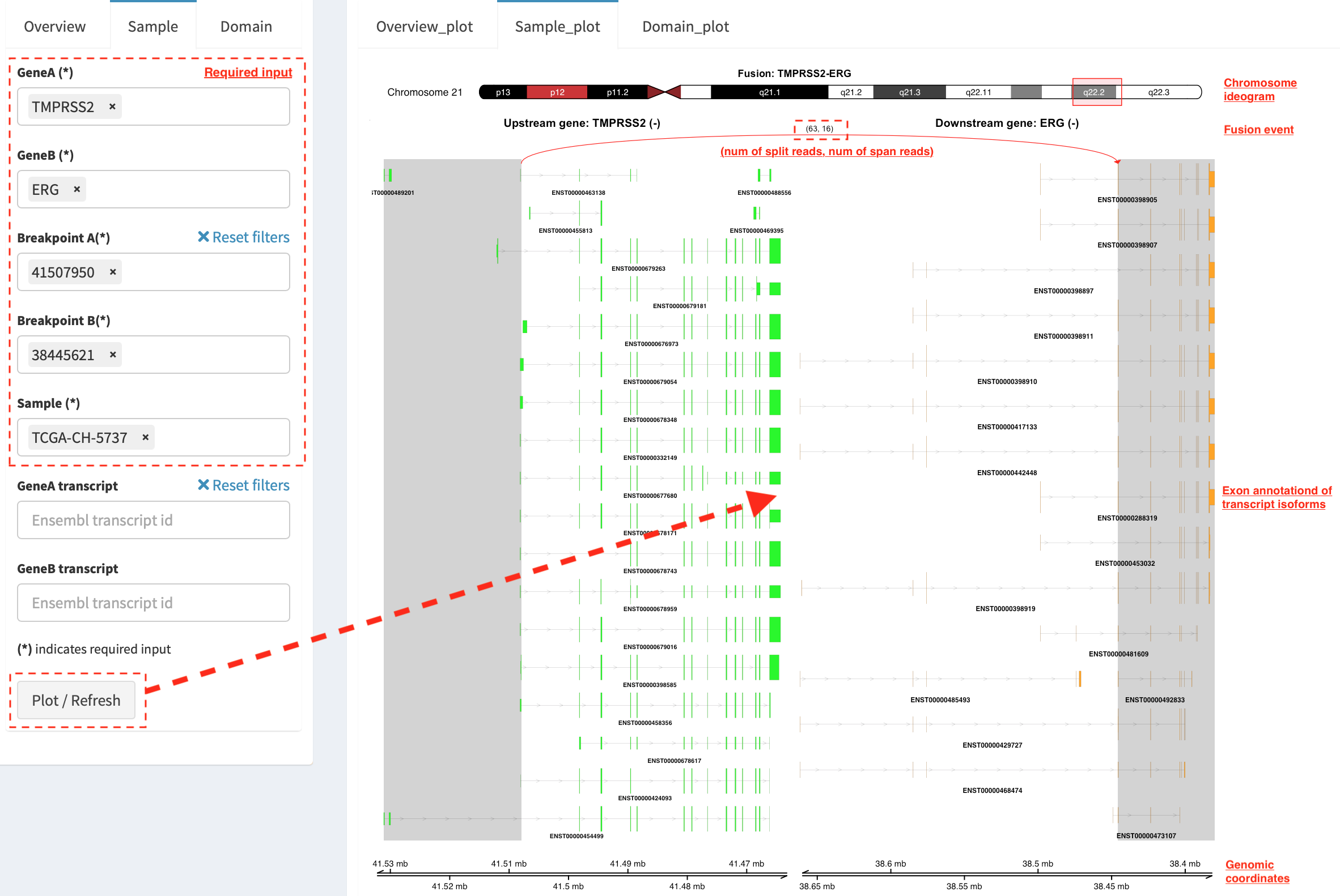
Overview_plot (only available for RNA-seq SVs)
It displays all fusion events related two partner genes and their
prevalence in a sample cohort. For example, choose partner gene names
(e.g. TMPRSS2 and ERG) in Select boxes GeneA (*) and
GeneB (*), and press Plot / Refresh. The two-way plot from the
top illustrates fusion events (curved lines with frequency in brackets),
exon annotations of different transcript isoforms for upstream (colored
by green) and downstream (colored by orange) partners, genomic
coordinates of partner gene loci in Mb from chromosome, partner gene
position in a chromosome ideogram.
Show fusion events of chosen breakpoints in Select boxes
Breakpoint A and Breakpoint B. For example, breakpoint
41507950 of TMPRSS2 is chosen; three fusion events with a
frequency (3, 42 and 17) are plotted on the top of two-way
plot view (highlighted in dashline box).
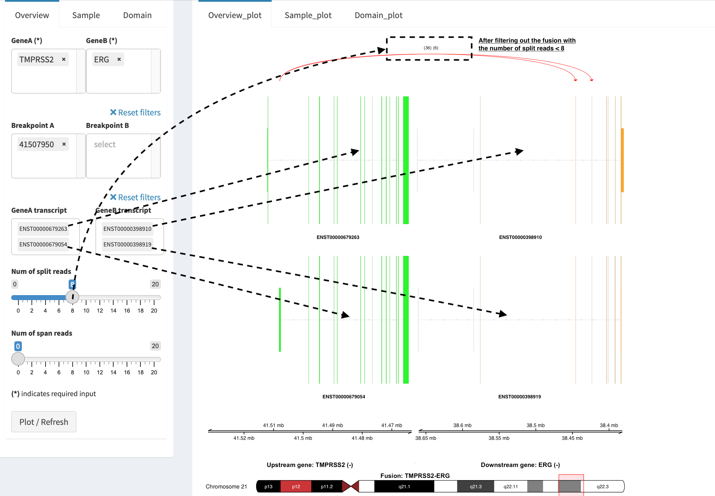
Show annotations of chosen transcripts in Select boxes
GeneA transcript (ENST00000679263 and ENST00000679054) and
GeneB transcript (ENST00000398910 and ENST00000398919), and
filter out the fusion event with the number of split reads less than 8
(see the setting of Num of split reads slider).
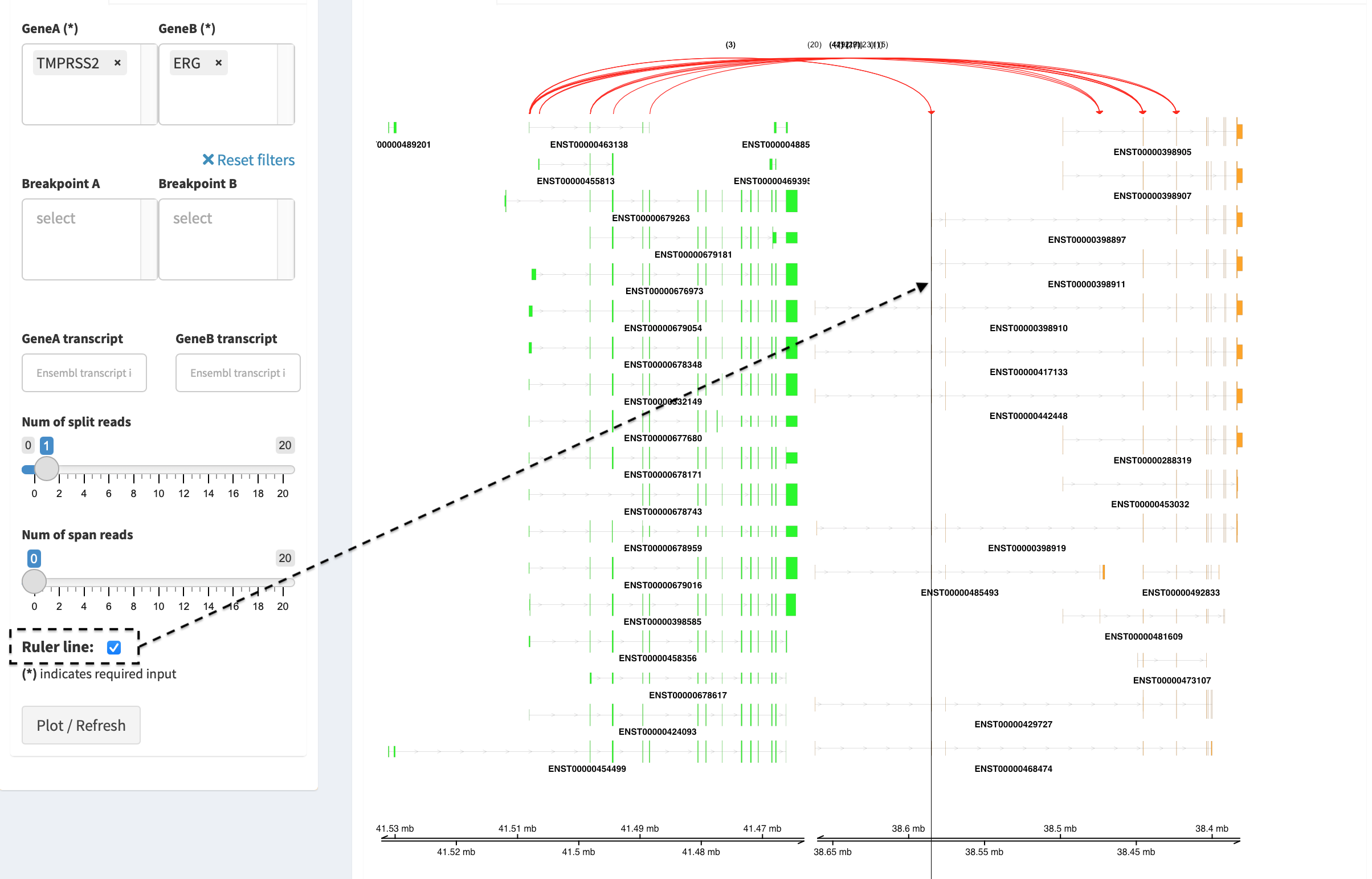
By clicking check box Ruler line:, users could add a vertical
baseline to the session in context of ‘exon-intron’ structure for
different transcript isoforms.
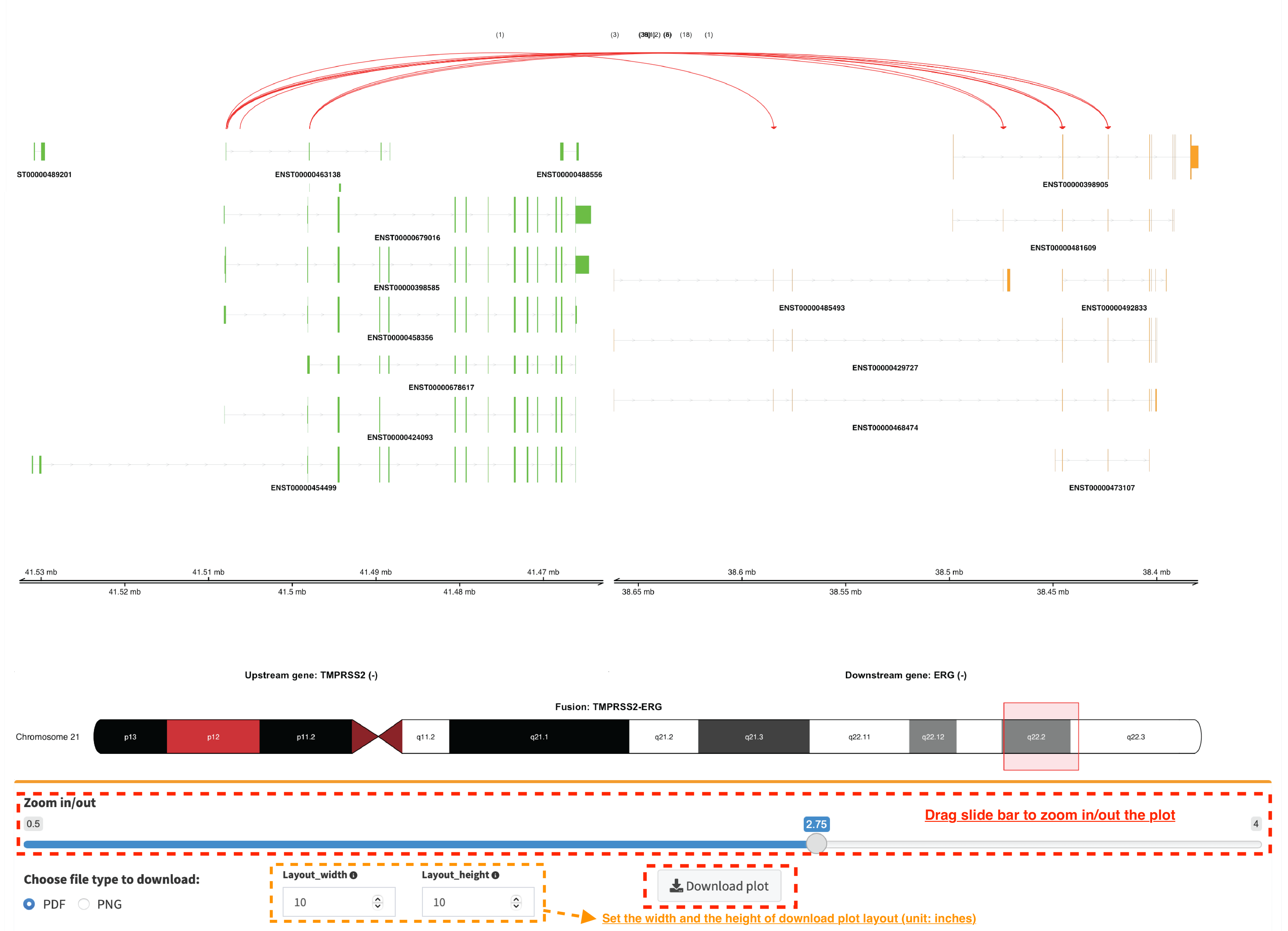
Zoom in/out and download plot, and users are able to adjust the
resolution of download plot via changing Layout_width and
Layout_height.
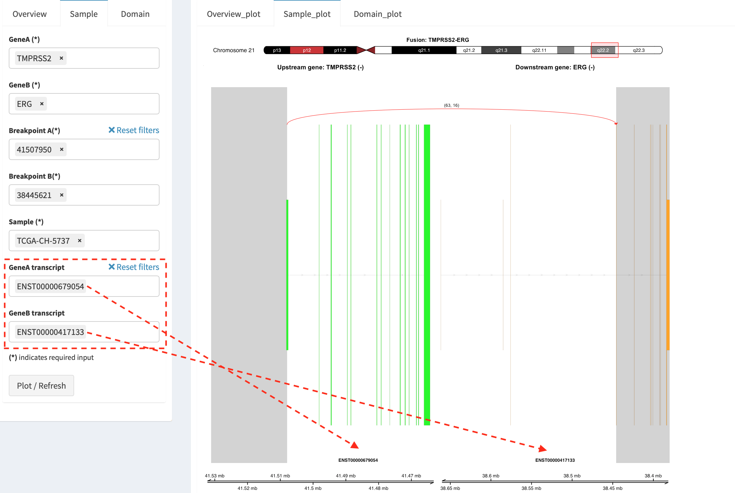
Sample_plot (only available for RNA-seq SVs)
It illustrates a private fusion event between two partner genes of one
sample in context of transcript isoform annotations. To make a plot, the
GeneA, GeneB, Breakpoint A, Breakpoint B and Sample
must be selected. For example, the demo case from the top shows the
position of partner genes in a chromosome ideogram, the fusion event
(the numbers of split reads and discordant read pairs are displayed in
the bracket above the curve), exon annotations of different transcript
isoforms for upstream (colored by green) and downstream (colored by
orange) partners in which fused parts are highlighted by grey box,
and genomic coordinates of partner gene loci in Mb from chromosome.
As a breakpoint may have a variable consequence (e.g. ‘at exon
boundary’, ‘within exon’ or ‘within intron’) in terms of different
transcript isoforms, users can choose the most relevant transcript in
Select boxes GeneA and GeneB transcript
(e.g. ENST00000679054 and ENST00000417133) to demonstrate the
outcome of fusion event.
For plotting read coverage using alignment file in a single sample analysis, see Appendix section.
Domain_plot (only available for RNA-seq SVs)
Domain plot shows a biological consequence of chimeric transcript in
context of protein domain and motif annotations. For example, after
choosing partner genes (TMPRSS2 and ERG) in Select boxes GeneA
and GeneB, transcript isoforms with domain and motif annotations are
bold and the canonical transcript isoform is highlighted by underscore
in Select boxes TranscriptA and TranscriptB. Choose relevant
ones, then domain fusion plot is rendered.
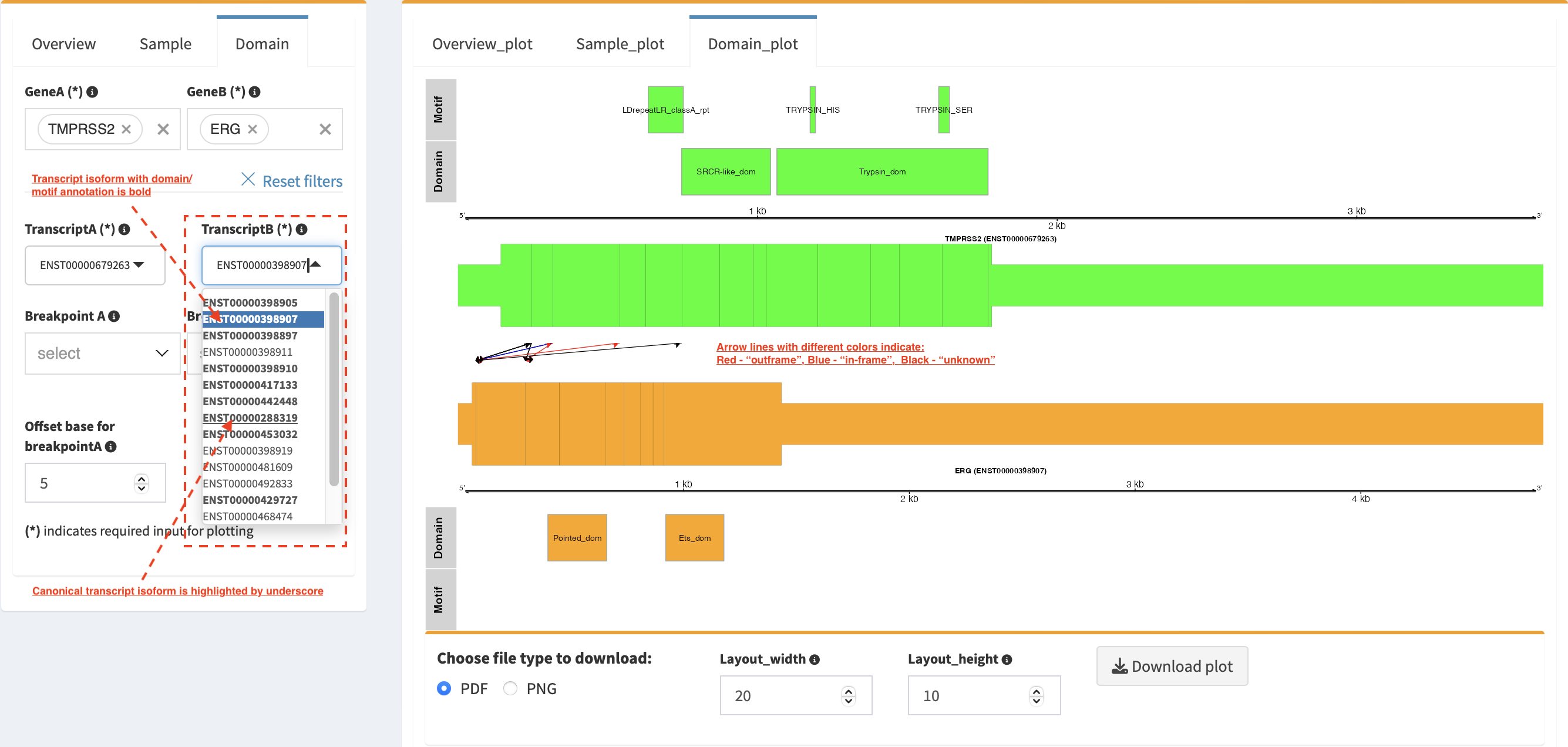
In plot view panel, motif & domain annotations and the selected
transcripts with concatenated exons for GeneA (colored by green) and
GeneB (colored by orange) are shown in upper and lower parts of the
layout, respectively. Colored arrow lines denote different biological
consequence of translated chimeric transcripts (i.e. red: outframe,
blue: inframe and black: unknown).
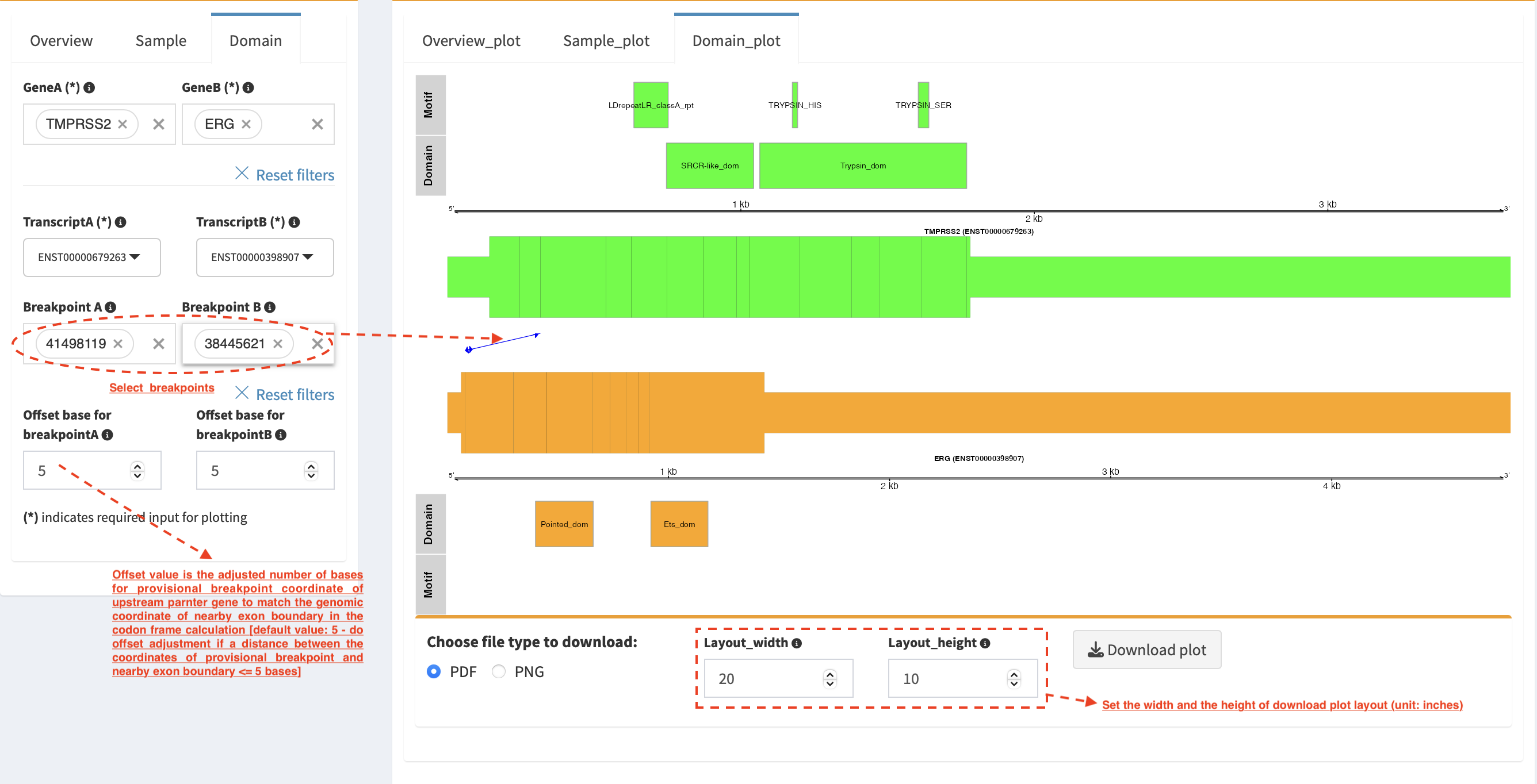
Show biological consequence of a specific chimeric transcript with the
selected breakpoints (e.g. 41498119 and 38445621 are chosen in
Select box Breakpoint A and Breakpoint B, see below). Users
could adjust the resolution of download domain fusion plot via changing
Layout_width and Layout_height.
Network module
The aim of this module is to identify a hub (i.e. a node with a high
degree of connection) in SV interaction network and reveal the impact of
SV events on functionality of involved genes. In the network, node
represents either a gene or an intergenic interval that harbors
breakpoints of SV, while edge shows a SV event between two nodes. The
results are presented in four functional panels
(RNA_SV_network_plot, RNA_SV_network_hub,
DNA_SV_network_plot and DNA_SV_network_hub).
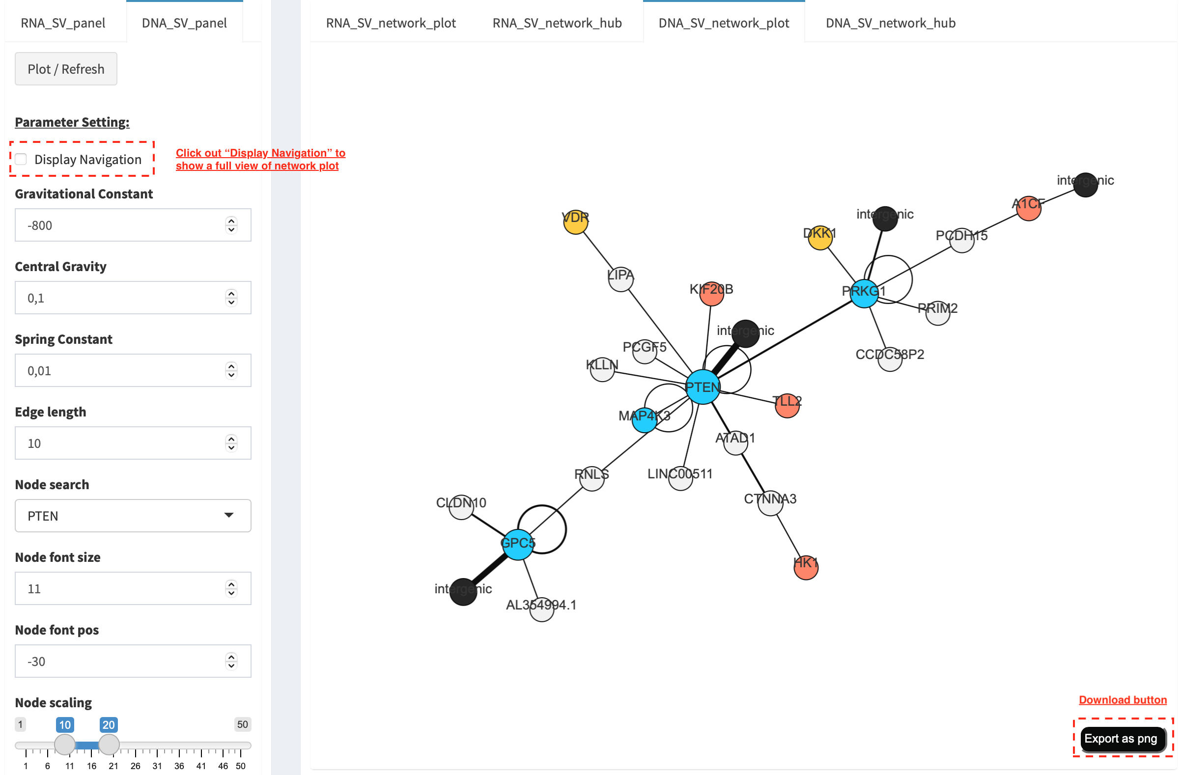
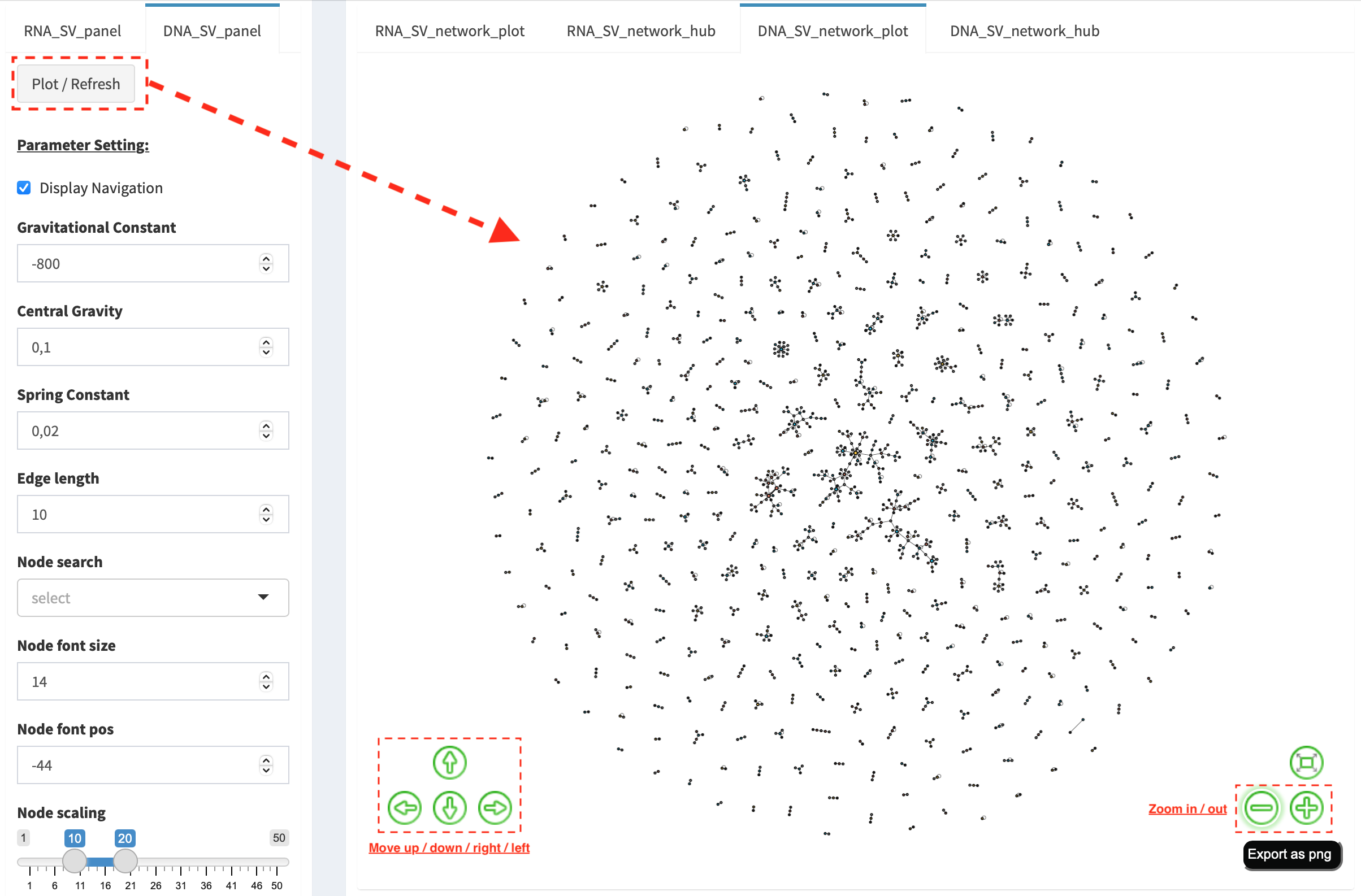
DNA_SV_network_plot
Press Plot / Refresh button in DNA_SV_panel settings. An
overview of DNA SV interaction network is plotted.
Choose a gene name (e.g. TP53) in Select box Node search of
DNA_SV_panel, and TP53 is centralized by its connected nodes. The
degree of TP53 (which is listed in DNA_network_hub panel) suggests
a structural variation complexity in the sample cohort. All nodes are
marked by five different colors (red: oncogenes,
blue: tumor suppressor genes, orange: cancer-related genes,
grey: the other genes and black: intergenic). In terms of a
tumor suppressor feature and a high degree of connection, an outcome of
SVs involving TP53 most likely results in a loss of function by
disrupting the gene.
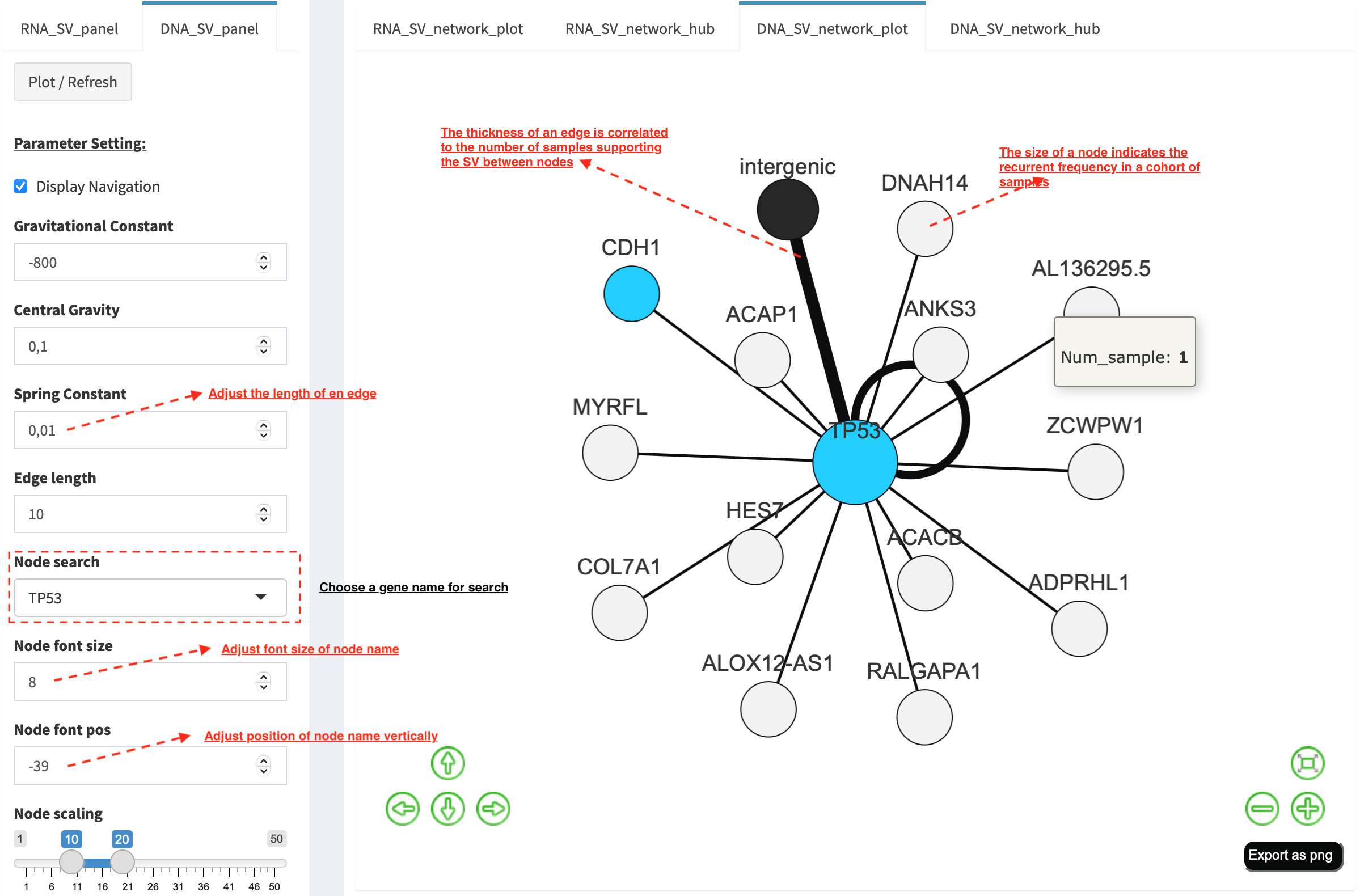
The gene name pops up after clicking a node in the network plot. User
could adjust font size and position of gene name using Numeric Input box
Node font size and Node font pos of DNA_SV_panel. The
thickness of an edge indicates the number of samples supporting a SV
event between nodes, and mouse over an edge pops up a windonw with the
sample number (e.g. Num_sample: 1). The length of edge is adjusted
by Numeric Input box Spring Constant (i.e. a smaller value suggests
a longer edge).
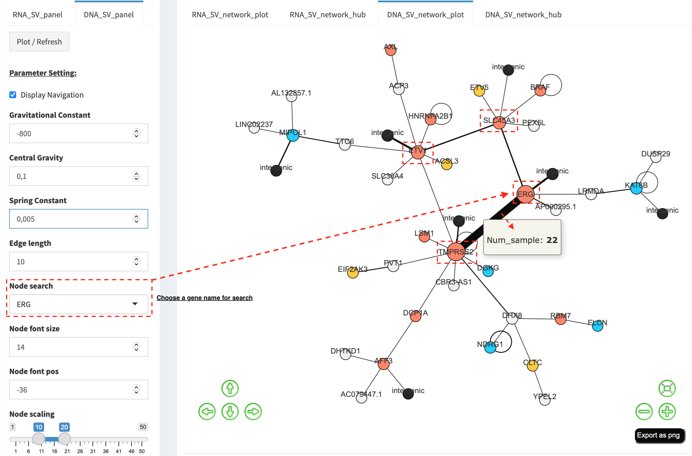
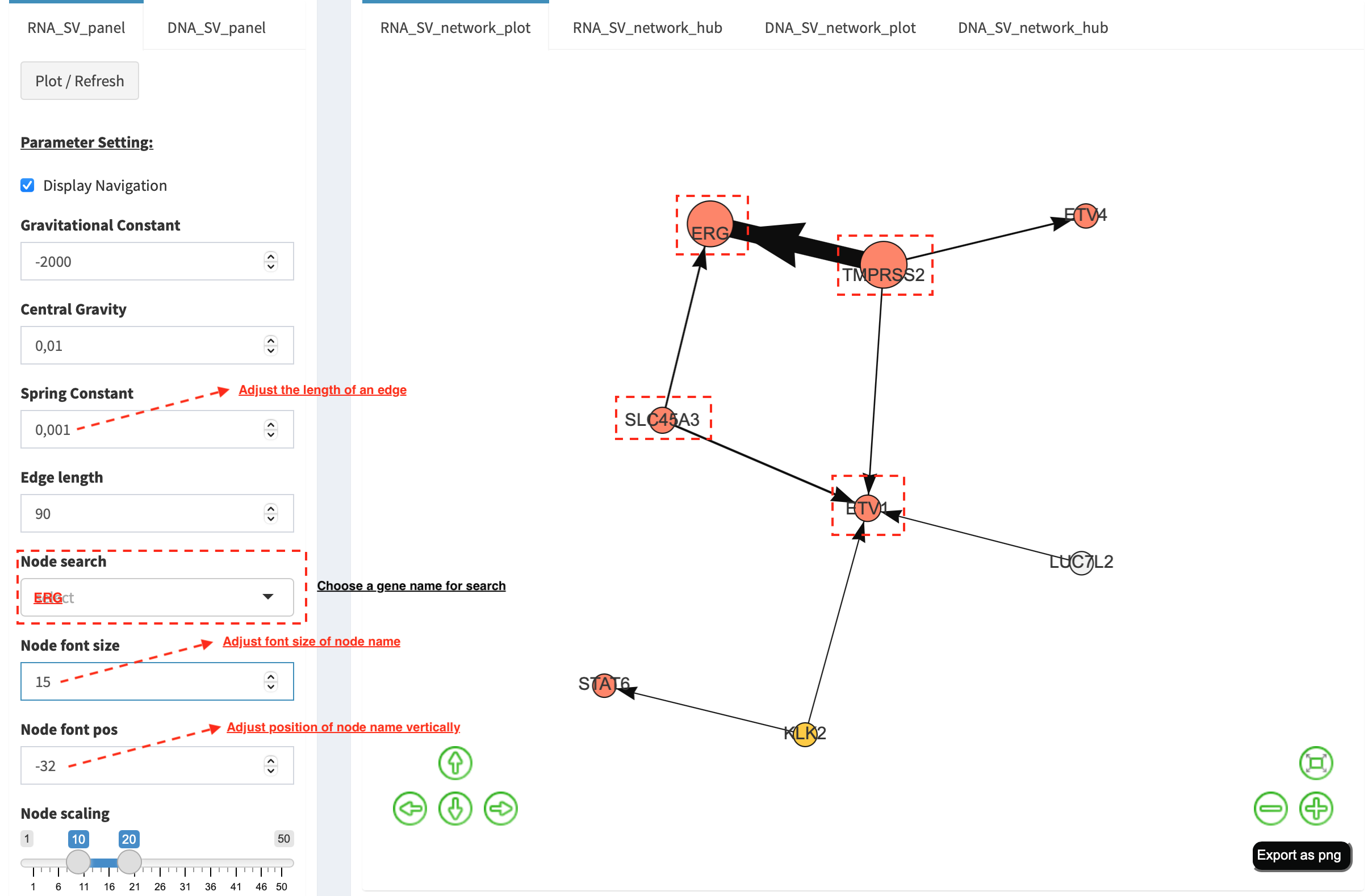
For another example, choose ERG in Select box Node search, and a
more complex sub-network is plotted. In addition to ERG, three other
hubs (ETV1, SLC45A3 and TMPRSS2) with a degree of 8, 6 and 10 (see
DNA_SV_network_hub panel) are highlighted in dash boxes. They are
enriched in SVs and highly interact with each other, which consists of a
functional module. Of them, the TMPRSS2-ERG shows a presence in 22
samples (see a pop-up window). As all the four hubs have oncogenic
features, and it is interesting to see whether such a interative network
can be recurrent at RNA level.
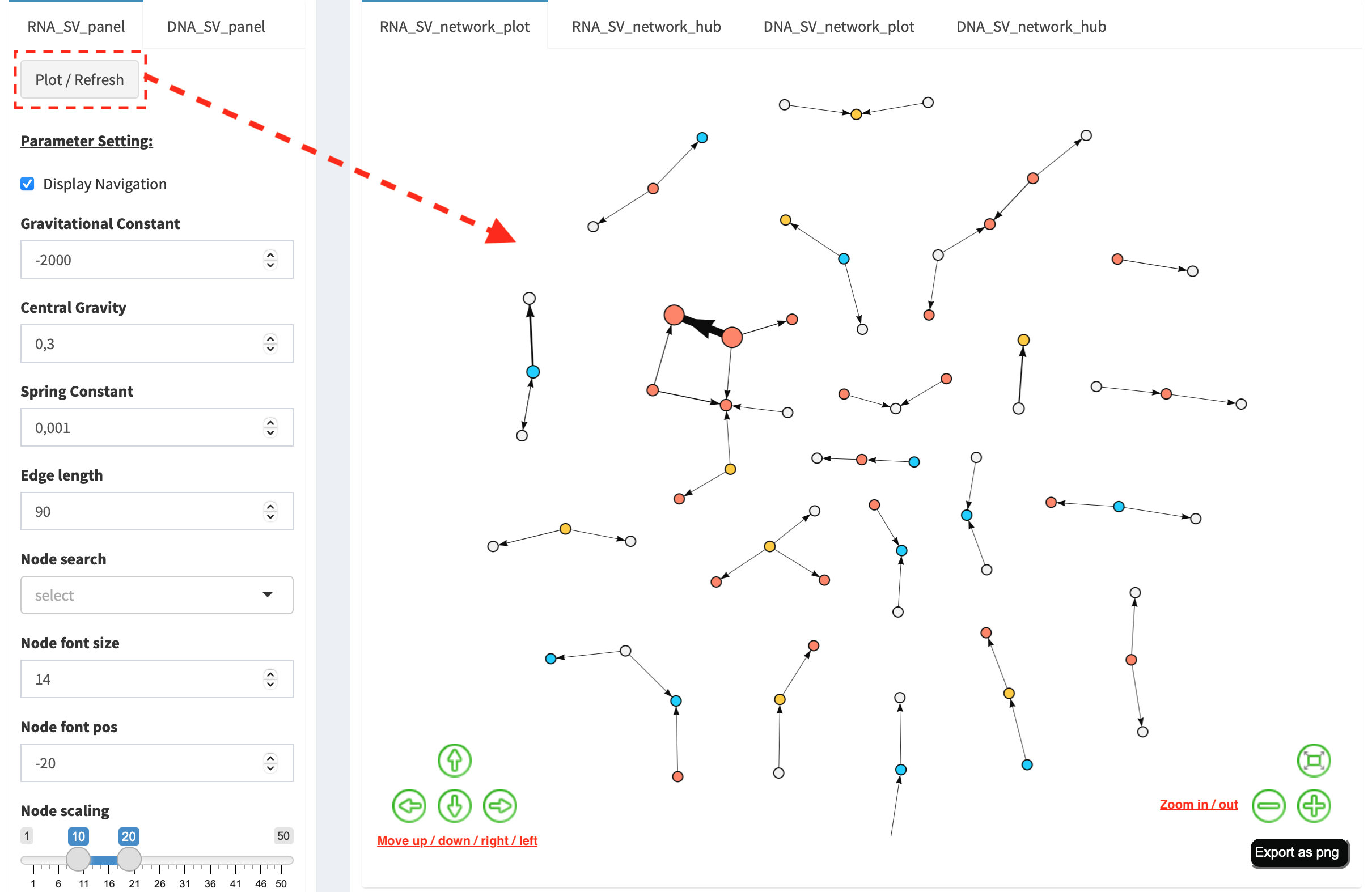
RNA_SV_network_plot
Press Plot / Refresh button in RNA_SV_panel. An overview of RNA
SV interaction network is plotted, which looks very similar to the
DNA_SV_network_plot except for edges with arrow lines. As most SV
events observed at RNA level are transcribed as fusion transcripts, an
arrow indicates the transcription direction from upstream to downstream
partner.
Choose ERG in Select box Node search of RNA_SV_panel, and the
sub-network with centralized ERG is highlighted. A similar subgraph
with the same hub composition (ERG, SLC45A3, ETV1 and TMPRSS2
colored as oncogenes) recurs. Arrows denoate the transcription
direction from upstream partners (TMPRSS2 and SLC45A3) to downstream
partners (ERG and ETV1), which might result in an increase of ERG
and ETV1 expression due to a “hitchhiking effect” of overexpressed
TMPRSS2 and SLC45A3.
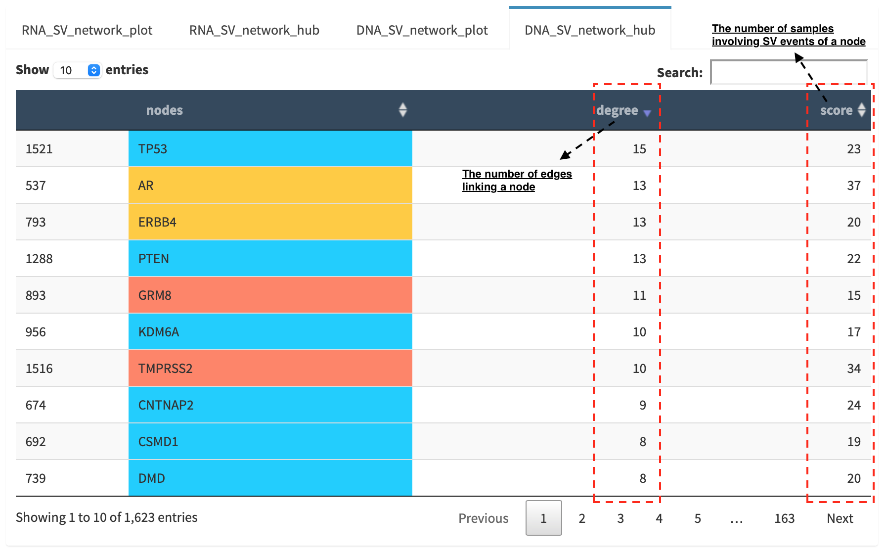
DNA_SV_network_hub and RNA_SV_network_hub
A table is generated to summarize network centrality/hub score. The
nodes column is marked by three colors (red: oncogenes,
blue: tumor suppressor genes and orange: cancer-related genes).
Two different values, degree and score, represent the number of
edges linking to a node and the number of samples involving SV events
for a node. By ranking table via degree and score, users could
identify the hub with a high complexity.
Download
The network is saved as png format by pressing Export as png button.
In order to download a full view of plot, Display Navigation could
be clicked out .