Appendix¶

Although FuSViz is designed for interpretation and visualization of SVs in a sample cohort, it can be utilized for single sample analysis together with read alignments as well. Read alignments from DNA-seq and RNA-seq data are able to be imported in Linear and Two-way modules.

Quality control of SVs via read alignment in Linear module¶

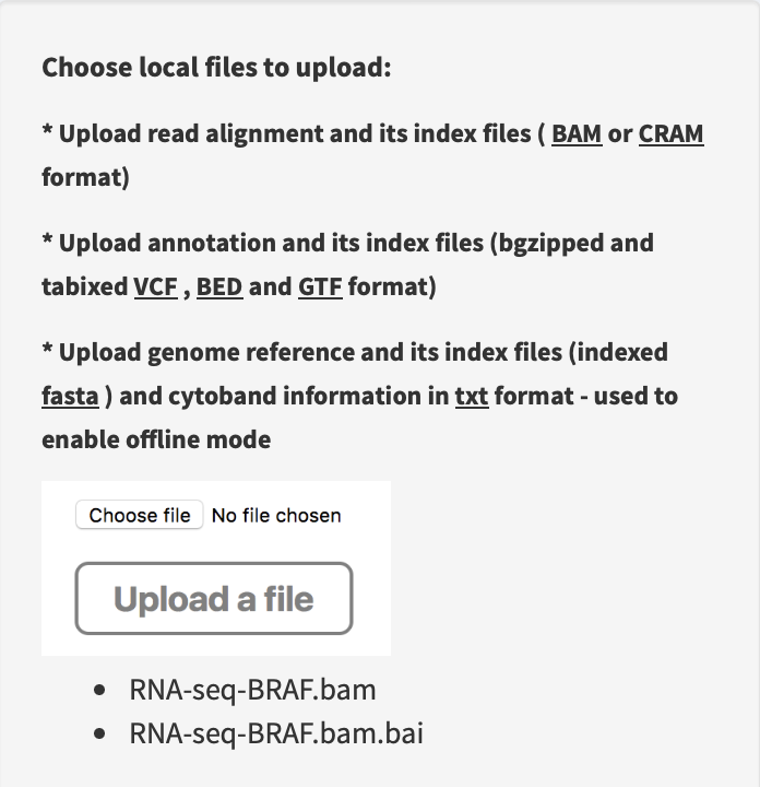
Load annotation resource data of human genome hg19 version, then upload RNA-seq alignment and index files at the path ~/inst/example/RNA-seq-BRAF.bam and ~/inst/example/RNA-seq-BRAF.bam.bai of FuSViz package.

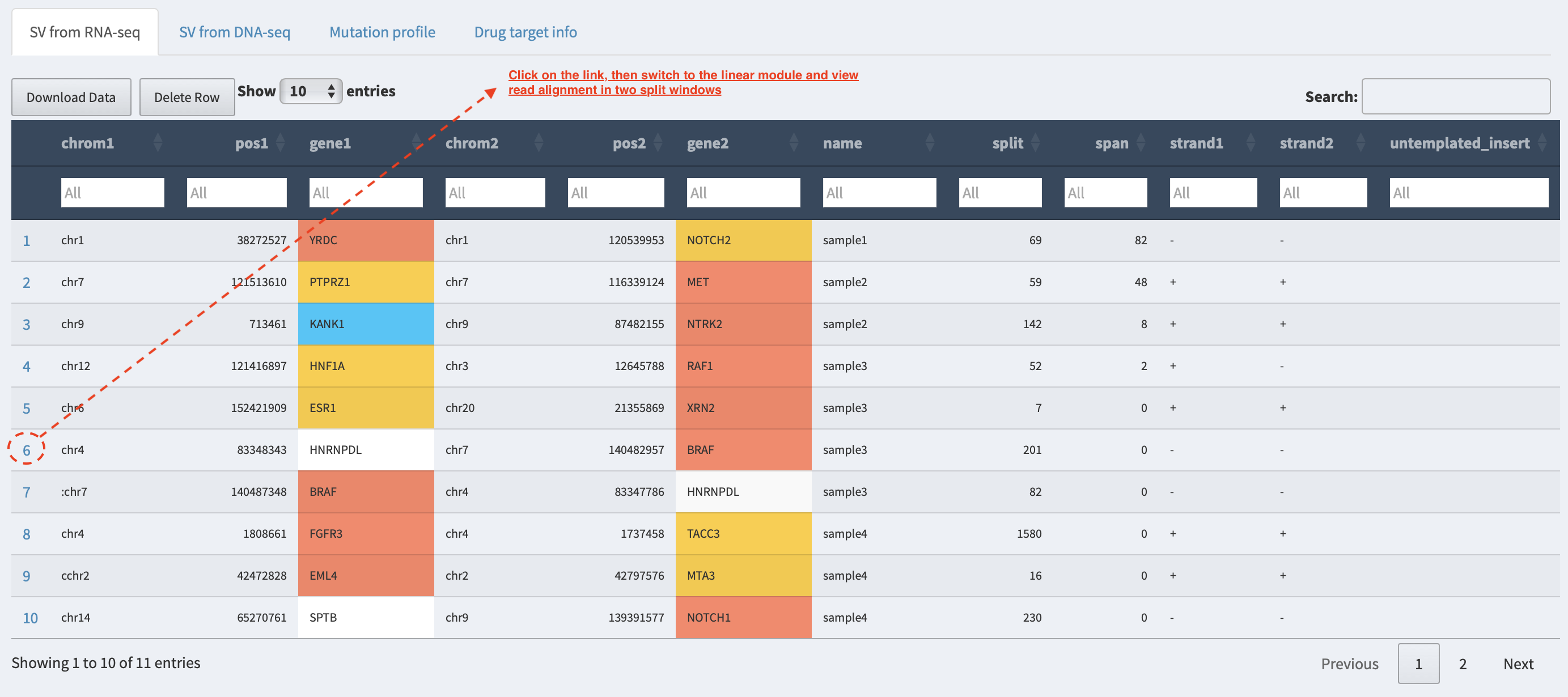
Import an example file of RNA SV calls at the path ~/inst/example/BRAF_demo.txt of FuSViz package. Click on the index of the 6th row (i.e., HNRNPDL-BRAF) that links to the linear view session, then genomic coordinates of HNRNPDL and BRAF breakpoints are shown in two split windows.

Inspect read alignment and search for supporting split reads at the breakpoints.

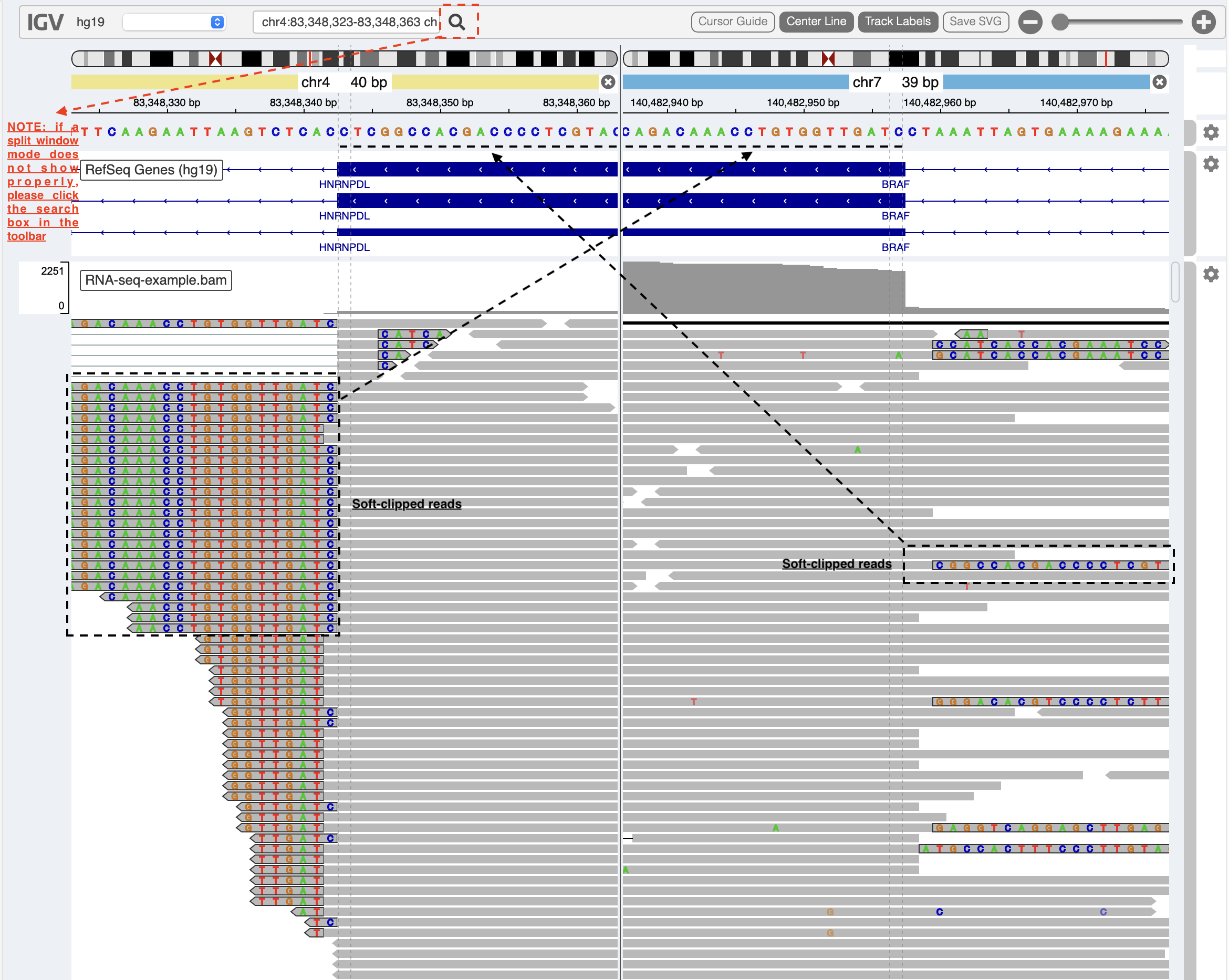
A split-window mode is used to investigate alignment quality of split reads mapped to HNRNPDL and BRAF genes (NOTE: please click on the search box in the toolbar if a split-window mode does not show properly). Soft-clipped read sequences (black box) match exactly the fusion sequences at breakpoints of the partner genes HNRNPDL and BRAF (black dash lines), respectively. Sometimes, the genomic coordinates of breakpoints need an adjustment if the provisonal ones are inaccurate.

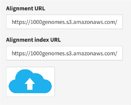
Load alignment track from URL address in Linear module¶

If alignment data is hosted in a remote server or a cloud, users can load it via URL web address. For example,

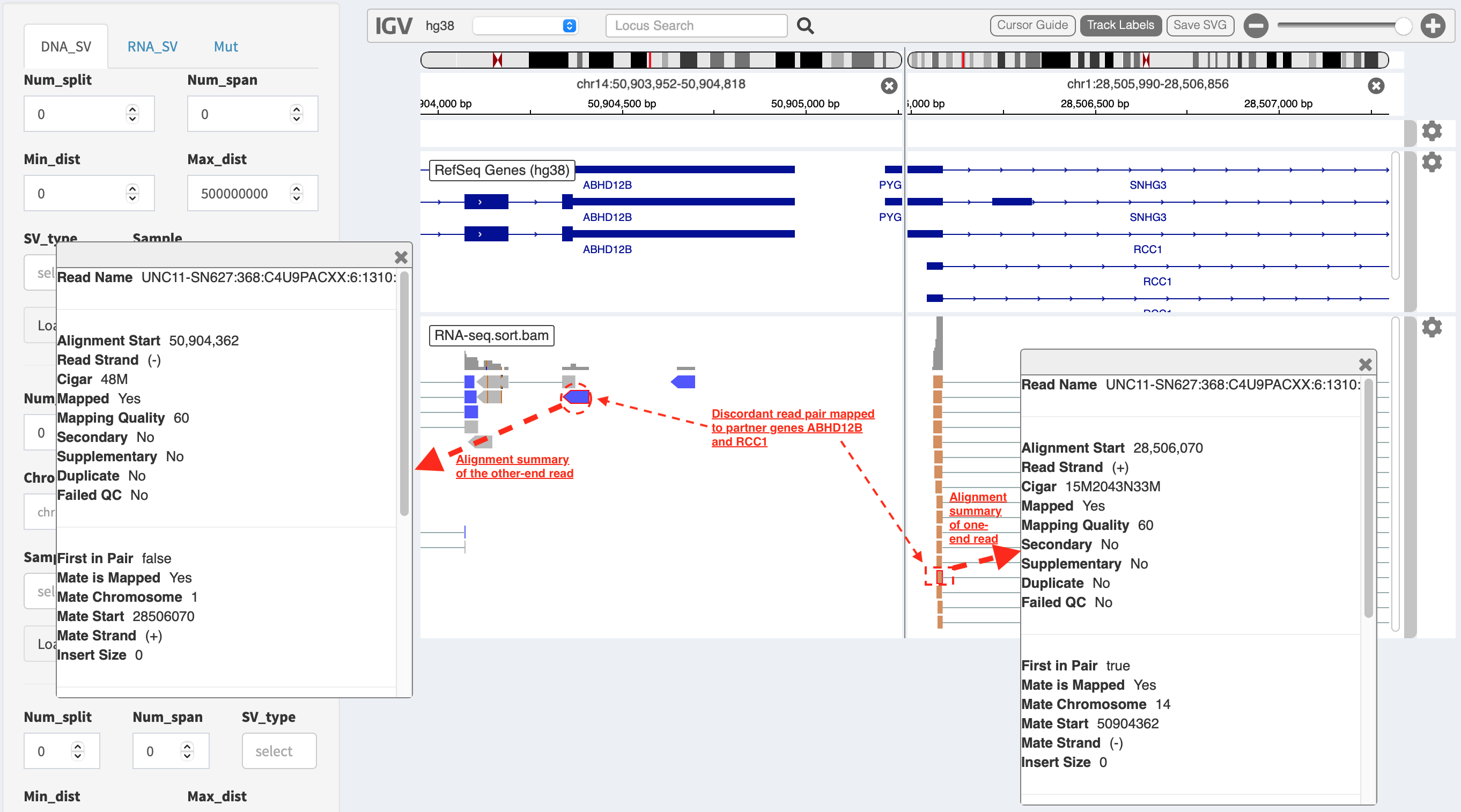
A split-window mode is also able to evaluate alignment quality of discordant read pairs mapped to different genomic loci. For another example, a read pair highlighted in dash boxes shows a discordant mapping feature to partner genes ABHD12B and RCC1, respectively.

Visualize SV event together with read coverage using Two-way module¶

This functionality is performed under CLI environment (NOT available via web interface). Firstly, load FuSViz package in R:

library(FuSViz)
options(uscsChromosomeName=FALSE)

Set gene/transcript annotation version (e.g. hg19) and RNA-seq alignment path

version = "hg19"; # or “hg38”
rna_bam_path=file.path(extdata = system.file("extdata", package = "FuSViz"), "RNA-seq-example.bam")

Use ‘plot_separate_individual_bam’ to visualize fusion together with RNA-seq read coverage¶

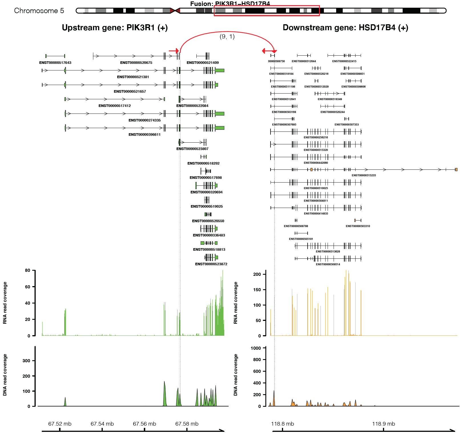
For example, plot a fusion event of “PIK3R1-HSD17B4”

plot_separate_individual_bam(first_name = "PIK3R1", second_name = "HSD17B4", breakpoint_A = 67576834, breakpoint_B = 118792010, coverage_plot_trans = F, version=version, rna_bam_path = rna_bam_path, split = 9, span = 1, fusion_strandA="+", fusion_strandB="-")

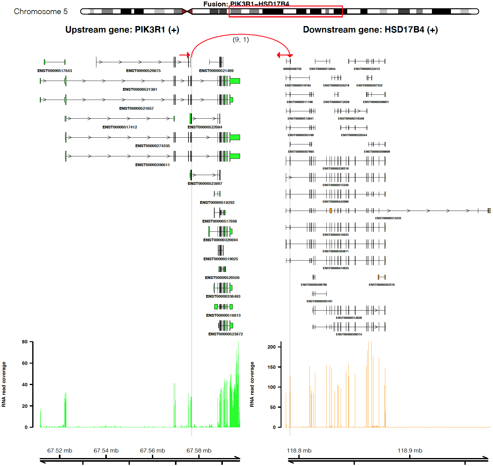
From the top it shows the position of partner genes in a chromosome ideogram, the fusion event (a curved line marked by read support [9 - split read, 1 – spanning read pair]; arrow indicates transcription direction of the fusion), exon annotations of different transcript isoforms for upstream (colored by green) and downstream (colored by orange) partners, RNA expression level measured by read counts and genomic coordinates of partner gene loci in Mb from chromosome. coverage_plot_trans = F suggests RNA read coverage is plotted using reads mapped to exons and introns of all transcript isforms of geneA and geneB.

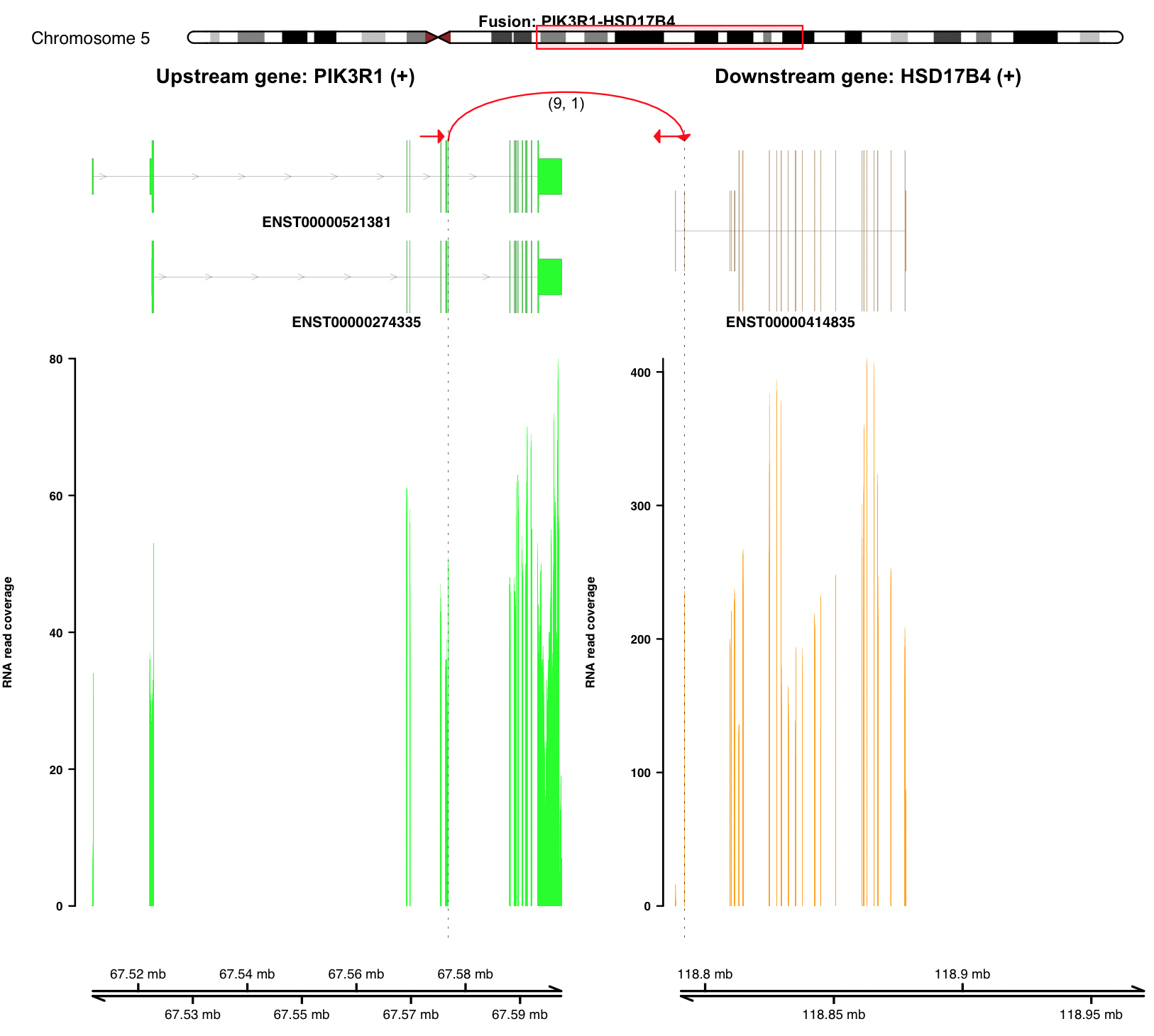
Visualize fusion and read coverage calculated using specific transcript isoforms¶

plot_separate_individual_bam(first_name = "PIK3R1", second_name = "HSD17B4", breakpoint_A = 67576834, breakpoint_B = 118792010, coverage_plot_trans = T, version=version, rna_bam_path = rna_bam_path, transcriptA="ENST00000521381 ENST00000274335", transcriptB="ENST00000414835", split = 9, span = 1, fusion_strandA="+", fusion_strandB="-")

coverage_plot_trans = T suggests RNA-seq read coverage is plotted using the exons of selected transcripts ENST00000521381 and ENST00000414835. If breakpoint falls within a intron, read coverage of the related intron is plotted as well.

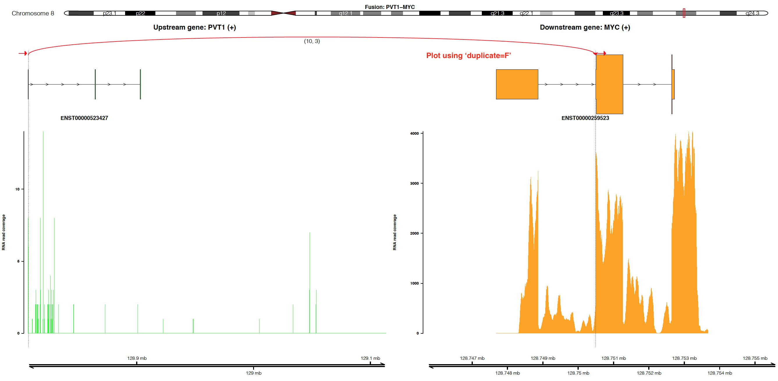
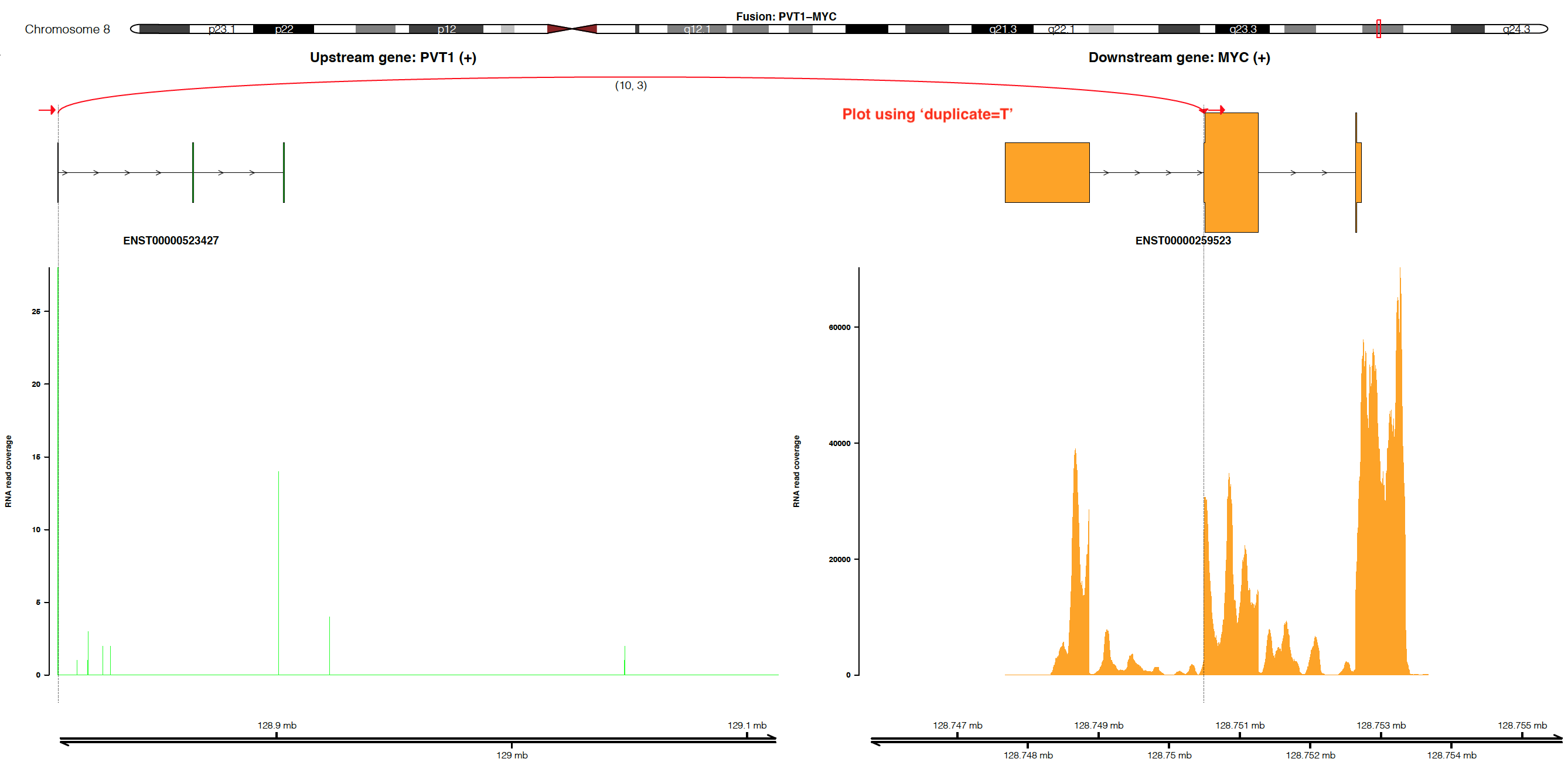
Visualize fusion and read coverage calculated by duplicated aligned reads¶

By default, the coverage is plotted using un-duplicated aligned reads (i.e. duplicate=F). If users would like to plot coverage using duplicated aligned reads, please set duplicate=T (NOTE: duplicate=T only works when alignment is processed by Picard or Samtools with the setting MarkDuplicate=T).

Visualize fusion if DNA-seq read coverage is available¶

dna_bam_path=file.path(extdata = system.file("extdata", package = "FuSViz"), "DNA-seq-example.bam");
plot_separate_individual_bam(first_name = "PIK3R1", second_name = "HSD17B4", breakpoint_A = 67576834, breakpoint_B = 118792010, coverage_plot_trans = F, version=version, chrom_notation_rna = T, chrom_notation_dna = F, split = 9, span = 1, rna_bam_path = rna_bam_path, dna_bam_path = dna_bam_path, fusion_strandA="+", fusion_strandB="-")

Read alignment from DNA-seq data can be whole genome sequencing, Exome-seq or gene-panel target sequencing. chrom_notation_rna = T suggests the chromosome notation in RNA-seq alignment file is named like ‘chrX’ (i.e. UCSC syntax); chrom_notation_dna = F denotes the chromosome notation in DNA-seq alignment file is named like ‘X’ (i.e. ensembl syntax).

An example of fusion and read coverage plot using docker engine¶

version = 'hg19';
docker run --rm -v `pwd`:/data senzhao/fusviz_shiny_app:1.0 R -e "library(FuSViz); options(uscsChromosomeName=F); pdf(file='/data/fusion_plot.pdf', height=7, width=14); plot_separate_individual_bam(first_name='PIK3R1', second_name='HSD17B4', breakpoint_A=67576834, breakpoint_B=118792010, coverage_plot_trans = T, version='$version', rna_bam_path=file.path(extdata=system.file('extdata', package='FuSViz'), 'RNA-seq-example.bam'), transcriptA='ENST00000521381 ENST00000274335', transcriptB='ENST00000414835', split=9, span=1, fusion_strandA='+', fusion_strandB='-'); dev.off();"

NOTE: the ouptput file fusion_plot.pdf is generated at the current path pwd as the path pwd in host machine is binded to the volume path /data in the container.

A full usage of ‘plot_separate_individual_bam’¶

See reference, ?plot_separate_individual_bam